
Microsoft Excel is having so many unbelievable capabilities that are not instantly perceived. In which Conditional Formatting is one of the option.
Conditional Formatting is the tool that used to format the cell or a range in the specific condition. We can use this option on the value of the cell or value of formula, it means if you have formula in cell then we can specify the value in “Conditional Formatting” of if we have value in the range then we can use Conditional Formatting by describing the formula to highlight the values.
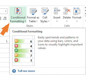
There are lot ways to use “Conditional Formatting” in our data. We can use it to show the numbers in increasing and decreasing order, to specific Value, to specific numbers, to specific date etc. Also we can highlight the cells by fill the color in cell, by change the font color, by using the data bars, color scales, icon sets.
What we are going to learn in this book?
Conditional Format Based on Dates
Find Occurrence of Text in a Column
How to Highlight a row on the basis of Cell
Compare 2 Columns and Return Fill Red if is different
How to check the row and then highlight the first cell of the row
Highlight Cells Tomorrow Excluding Weekend
Conditional Formatting to Mark Dates on a Calendar
How to apply Conditional Formatting in a Cell before a Particular Character
Highlight the Top 10 Sales through Conditional Formatting
Conditional Formatting for Pivot Tables
Conditional Format Between First and Last Non-Blank Cells
![]()
![]()
The applications/code on this site are distributed as is and without warranties or liability. In no event shall the owner of the copyrights, or the authors of the applications/code be liable for any loss of profit, any problems or any damage resulting from the use or evaluation of the applications/code.


Nice presentation...
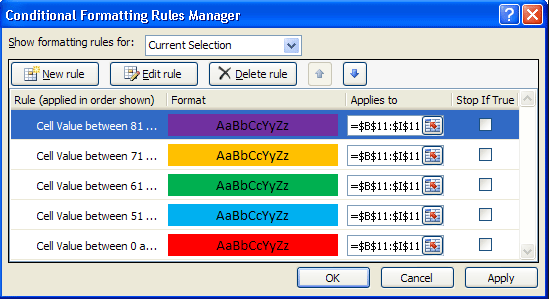
I use conditional formatting as part of a work-around I developed for working with dates before 1900. I could enter such dates as text, but then I couldn't do math with them. Instead I take advantage of the fact that the Gregorian calendar repeats every 400 years. 1776 becomes 2176, 1812 becomes 2212, etc. For consistency I do the same with dates after 1900. 1945 becomes 2345, 2015 becomes 2415, etc. I format the dates to display 2-digit years, then to tell the centuries apart I color-code the dates. The 1st half of the 18th century (values 73416 to 91677) is gray, the 2nd half of the 18th century (91678 to 109939) is purple, the 1st half of the 19th century (109940 to 128201) is blue, the 2nd half of the 19th century (128202 to 146463) is green, the 1st half of the 20th century (146464 to 164725) is yellow, the 2nd half of the 20th century (164726 to 182988) is orange, and the 1st half of the 21st century (182989 to 201250) is red.
Its good one.Thank you all for the effort done.
Good tips, from a technical standpoint.
But if you are going to publish tips in English then you should at least hire an editor whose native language is English.
Hi,
Thanks for your feedback. We will surely improve our content.
We're a small team at ExcelTip working hard to bring good stuff for you everyday.
Thanks,
Team Excel Tip & Excel Forum
It helped me do the needful in my job. It is a nice one.
All these examples would have more value if the formulae were explained. It's all very well doing things by rote, but if you can't understand the principles used then it is of little value.
Amazing!! Good Work Team!! Keep sharing it with us such amazing tricks 🙂 Looking forward to have something on Excel 2016. 🙂
Its a nice one