In this article, we will learn All about Drop down list in Excel.
Scenario:
Data Validation is the tool that is used to restrict the entry in a range or data so that we can define which type of data should be entered in the sheet. It guides the user to input the type of option which is necessary for your worksheet. Here the problem is, we need to input message as caution. We add a caution message to let the user know what values to enter. Let's learn more about Data validation input message in Excel here.
Access Data Validation in Excel
Go to Data > Data validation arrow > Data validation > Input title > Input message > Click Ok.
Note: You can also customize the warning message from the Error alert message.
Some of the most used features of Drop Down list.
Create a drop down list
All of these might be confusing to understand. Let's understand how to use the function using an example. First, let’s understand how to make a dropdown list in Excel with an example here

Here is a list of three colours Red, Green and Blue. We need to create a cell which takes only either of the values given from this list.
Click Data > Data Validation option in Excel

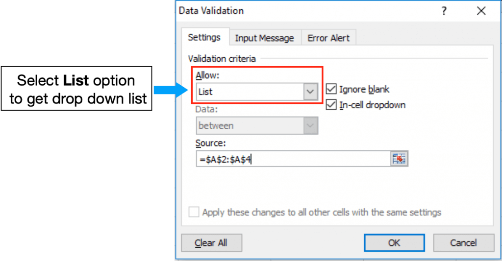
Data Validation dialog box appears as shown above.

Select the option List in Allow and select the source list in Source option and click OK.
A dropdown list will be created on the cell.

As you can see we have a cell C5 which shows only 3 given values to choose from.
Access Message box with drop down list
Here we will apply a data validation on the cell to allow the user to input any value which is a number. Below is the snapshot how to use data validation.

Here you noticed after Select Custom from Allow method list which allows you to use the formula in cell. Click Ok to apply.

We tried typing the text value as we enter a text value, it throws an error "This value doesn't match the data validation restrictions defined for this cell".
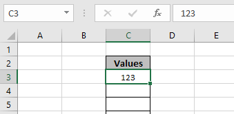
Now, we tried the number value in the cell and the cell accepts the number value as shown in the above image. You can also customize the error message and alert message to let users know what values are prohibited. Edit alert and message as shown below.

Input Alert message be typed in Input Message tab as shown in above image.

An Error Alert message be used in the Error Alert tab. Now click OK to get these changes.

As you can see the Caution alert in the yellow box hanging below C3 cell. Now you can copy the Data validation format to the rest of the required cell using Ctrl + D.

As you can see, now these cells can be used to allow numbers only. Now learn how to perform Data validation using VBA
Alternate way using VBA
We have countries’ names in the D column, and in cell A1, we want to create a drop down filter for countries’ names.
We want to highlight the cell A1 and make the drop down list to countries’ names and put the message to let the users know which entries need to be entered in the range.
Follow below given steps and code:-
Open the VBE page to press the key Alt+F11.
Insert the module to write the code.
Write the below mentioned code:-
| Sub DropDownFilter()
Dim lastrow As Long lastrow = Worksheets("sheet1").Cells(Rows.Count, "D").End(xlUp).Row With Range("A1:A10").Validation .Add Type:=xlValidateList, AlertStyle:=xlValidAlertStop, Operator:=xlBetween, Formula1:="=$D$2:$D" & lastrow .IgnoreBlank = True .InCellDropdown = True .InputTitle = "Message" .InputMessage = "Enter only countries name" Range("A1:A10").Interior.ColorIndex = 37 End With End Sub |

Add the code as shown above and press f5 from the keyboard to enable the change on the sheet.
First we had defined all the variables, then we had created the range which would help to create the dynamic drop down filter. Similarly, we had defined the input title and Input message. And then we had defined the destination where we wanted to create the drop down list and then we would fill the cell with color.
You can use a formula to allow text value only i.e. =ISTEXT(cel_ref). You can use any formula that returns True or False in the formula bar of the data validation tool.
Edit a drop down list
Here we have some lists here as shown below.

First, we need to create a dropdown list for the Main Category and then we will proceed to Sub_Category.
Select Formula>Name Manager in Defined names OR use shortcut Ctrl + F3 to open Name manager where we will keep lists of the array with their names so that we can call them by there name whenever required.

Click New to create. Here Name will be Month and in Refers to option enter the list under Month as shown below.

The same we will do for Week_Days and it will show like

Click Close and now select the cell where we need to add a dropdown list.

Then Click Data validation under Data bar. Choose list option is Allow and select the cells for main category names which in this case is at B2 and C2 cell “Month” and “Week_Days”
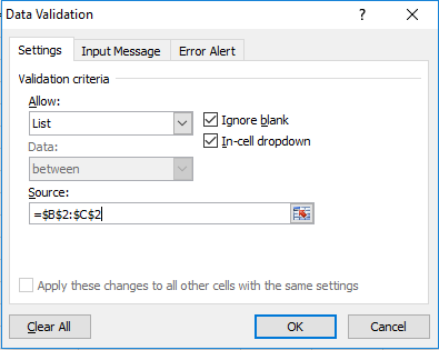

As we can see a drop down list is created which asks the user to choose from the given option.
Now select the cell under Sub_Category and just write the formula in Data validation and click OK.
Formula:
| =INDIRECT(E4) |

The result is displayed like this

If I don’t want Month and Week_Days. Instead, I want Fruits_Name and vegetables_Name. We just need to edit our Name Manager list.
Press Ctrl + F3 to open Name manager and delete the already inserted list and add new lists i.e. Fruits_Name and Vegetables_Name.

Now select the cell under Sub_category as shown in the snapshot below.
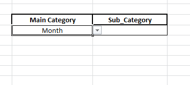
Instead of Month and Week_Days cell, we will use Fruits_Name and Vegetables_Name in Data Validation and click OK

As you can see the new list is added here.
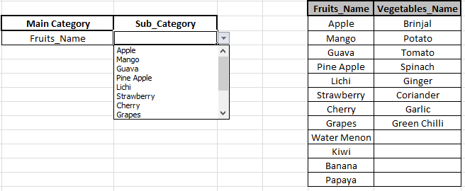
This is the way we can edit in the dropdown list and change the list selection.
Delete a drop down list
To delete or remove an already existed dropdown list. Just follow the simple steps as shown below.
Using Data validation option we can remove the dropdown list
We have a dropdown list here

Select the cell where you wish to remove the dropdown list.
Go to Data > Data Validation

Select Clear All option in the Data Validation dialog box and Click OK.

Now it's just the text written in that cell. You can edit that cell as the dropdown list is removed.
Drop down list which pulls data from different sheets
Here we take a example to understand better. Let's say you are a teacher. You have prepared attendance of students in a workbook. Each month’s attendance is in a different sheet of that month’s name.

In a master sheet, you want to put a VLOOKUP to check if that student was present or absent that month. It would be simple if your data was on the same sheet, but it is not. It is in different sheets. But it doesn’t mean we can’t pull data from another sheet in excel. We can and will.
For the month, you have created a drop down in cell C1. It contains a list of months. Now you want to show absent or present based on the selected month in Cell C1. Let's just see the generic formula first.
Generic Formula for VLOOKUP from Multiple Sheets:
| =VLOOKUP(lookupValue,INDIRECT("" & cell that contains name of month & "!range"),col_index_no,0) |
For this example, I have my attendance in “Jan”, “Feb”, and “Mar” sheets in the same range A2:C11.

Now I have prepared a master sheet.

In cell C4, put this formula and drag it down.
| =VLOOKUP(B4,INDIRECT(""&$C$1&"!B2:C11"),2,0) |
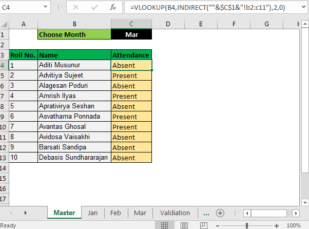
Now, whenever you change the month’s name in cell C1, excel will pull value from another sheet (from that month's sheet, if it exists).
Explanation :
We used the Excel Indirect function to fetch value from another sheet.
INDIRECT changes the text into reference.We used INDIRECT for referencing other sheets in excel.
For example, if you write INDIRECT(“sheet2:A2”) in a1 on sheet1. It will pull the value from sheet2!A2 in sheet1:A1. If you write =VLOOKUP(“abc”,INDIRECT(“sheet2!A2:B100”),2,0) any sheet,
VLOOKUP will look for “abc” in range A2:B100 on sheet2.
INDIRECT(""&$C$1&"!B2:C11") : Here we want the sheet name to change, that is why we have written it like this. If Cell C1 contains “Jan”, it will translate to INDIRECT(“Jan!B2:C11”) which will then translate to Jan!B2:C11 for VLOOKUP table array. If C1 has Feb it will translate to INDIRECT(“Feb!B2:C11”) and so on.
Afterwards, VLOOKUP did the remaining job.
VLOOKUP(B4,INDIRECT(""&$C$1&"!B2:C11"),2,0): now since Indirect gave the table array, VLOOKUP simply pulls data from that range easily.
Here are all the observational notes using the formula in Excel
Notes :
Hope this article about the Drop down lists in Excel is explanatory. Find more articles on calculating values and related Excel formulas here. If you liked our blogs, share it with your friends on Facebook. And also you can follow us on Twitter and Facebook. We would love to hear from you, do let us know how we can improve, complement or innovate our work and make it better for you. Write to us at info@exceltip.com.
Related Articles :
Data Validation in Excel : Restricts users to input value manually using this tool in Excel.
Way to use Vlookup function in Data Validation : Restrict users to allow values from the lookup table using Data validation formula box in Excel. Formula box in data validation allows you to choose the type of restriction required.
Restrict Dates using Data Validation : Restrict user to allow dates from a given range in cell which lays within Excel date format in Excel.
How to give the warning messages in Data Validation : Restrict users to customize input information in the worksheet and guide the input information through error messages under data validation in Excel.
Create Drop Down Lists in Excel using Data Validation : Restrict users to allow values from the drop down list using Data validation List option in Excel. List box in data validation allows you to choose the type of restriction required.
Popular Articles :
50 Excel Shortcuts to Increase Your Productivity : Get faster at your tasks in Excel. These shortcuts will help you increase your work efficiency in Excel.
How to use the VLOOKUP Function in Excel : This is one of the most used and popular functions of excel that is used to lookup value from different ranges and sheets.
How to use the IF Function in Excel : The IF statement in Excel checks the condition and returns a specific value if the condition is TRUE or returns another specific value if FALSE.
How to use the SUMIF Function in Excel : This is another dashboard essential function. This helps you sum up values on specific conditions.
How to use the COUNTIF Function in Excel : Count values with conditions using this amazing function. You don't need to filter your data to count specific values. Countif function is essential to prepare your dashboard.
The applications/code on this site are distributed as is and without warranties or liability. In no event shall the owner of the copyrights, or the authors of the applications/code be liable for any loss of profit, any problems or any damage resulting from the use or evaluation of the applications/code.