

In this article, we will learn How to compare two lists in Excel.
Color duplicate values in two lists in Excel
Given two different lists in Excel and we need to find items in one list which have its duplicate in another list. For example finding the employees who work in multiple departments. Excel Compare two columns and highlight duplicates values in given two lists.
Conditional formatting in Excel
Conditional formatting option allows you to highlight cells based on some given situation. Here we have to find duplicates in two lists. We have an option to highlight duplicate or unique values in Excel. Just follow the steps to solve the problem.
Example :
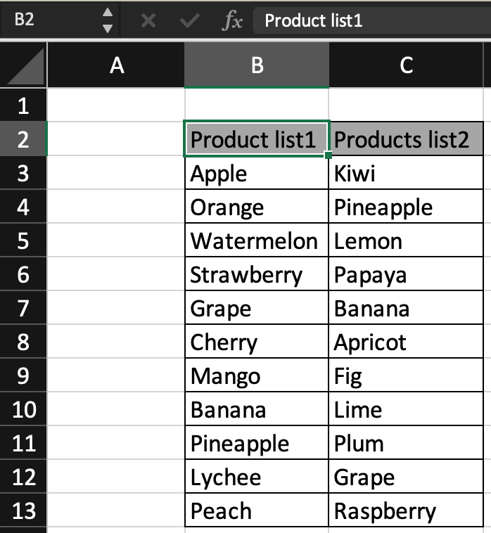
All of these might be confusing to understand. Let's understand how to use the function using an example. Here we have two lists of products to buy. But we don't need to buy duplicate entries of products which are in the other list. So the conditional formatting option enable excel to highlight cells with duplicate values in other list.
Follow the steps as explained below
Select the both lists using select and drag from mouse or using keyboard shortcut.
Go to Conditional formatting > Highlight cell rules > Duplicate values...

Duplicate Values dialog box appears. Select the duplicate option from the drop down list and highlight style from the other drop down list.
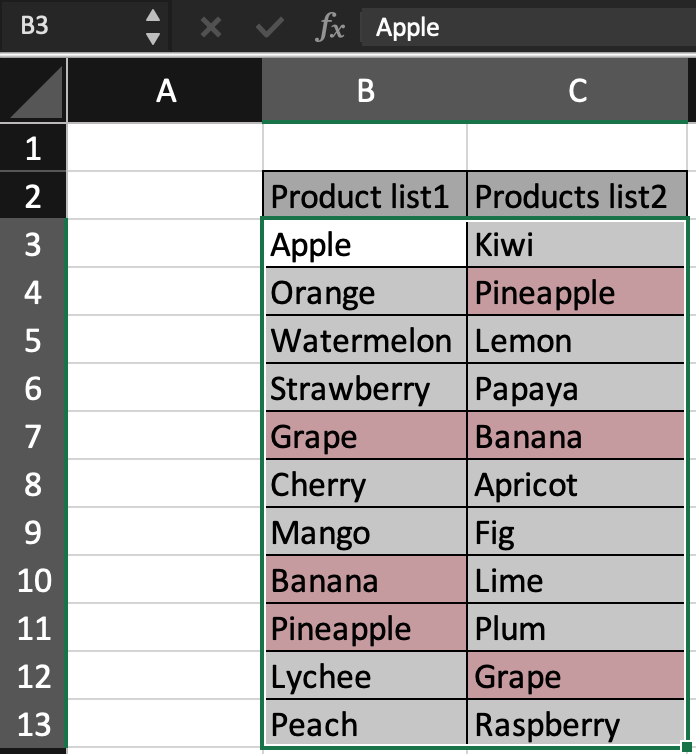
As you can see all the products which have some duplicate are highlighted. You can also highlight only unique values in Excel
Highlight unique values in two lists
Just consider it from the same above example. If We need to highlight only the products which have no duplicate in other lists.
Follow the steps as explained below
Select the both lists using select and drag from mouse or using keyboard shortcut. Then Go to Conditional formatting > Highlight cell rules > Duplicate values...
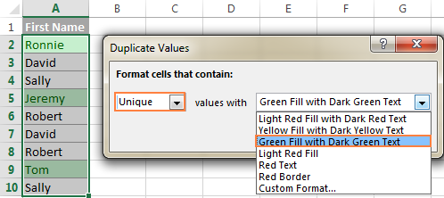
Duplicate Values dialog box appears. Select the unique option from the drop down list and highlight style from the other drop down list.
Press Enter and your unique value cells will be highlighted as shown below.

All the Green Highlighted cells have unique values. You can also clear out these highlighted cells.
Select the cells where need to clear these highlighted coloring. Just go to Conditional formatting > clear rules on Selected cell. That ought to do it
Here are all the observational notes using the conditional formatting in Excel
Notes :
Hope this article about How to compare two lists in Excel is explanatory. Find more articles on coloring and highlighting cells and related Excel formulas here. If you liked our blogs, share it with your friends on Facebook. And also you can follow us on Twitter and Facebook. We would love to hear from you, do let us know how we can improve, complement or innovate our work and make it better for you. Write to us at info@exceltip.com.
Related Articles :
Find the partial match number from data in Excel : find the substring matching cell values using the formula in Excel
How to Highlight cells that contain specific text in Excel : Highlight cells based on the formula to find the specific text value within the cell in Excel.
Conditional formatting based on another cell value in Excel : format cells in Excel based on the condition of another cell using some criteria.
IF function and Conditional formatting in Excel : How to use IF condition in conditional formatting with formula in excel.
Perform Conditional Formatting with formula 2016 : Learn all default features of Conditional formatting in Excel
Conditional Formatting using VBA in Microsoft Excel : Highlight cells in the VBA based on the code in Excel.
Popular Articles :
How to use the IF Function in Excel : The IF statement in Excel checks the condition and returns a specific value if the condition is TRUE or returns another specific value if FALSE.
How to use the VLOOKUP Function in Excel : This is one of the most used and popular functions of excel that is used to lookup value from different ranges and sheets.
How to use the SUMIF Function in Excel : This is another dashboard essential function. This helps you sum up values on specific conditions.
How to use the COUNTIF Function in Excel : Count values with conditions using this amazing function. You don't need to filter your data to count specific values. Countif function is essential to prepare your dashboard.
The applications/code on this site are distributed as is and without warranties or liability. In no event shall the owner of the copyrights, or the authors of the applications/code be liable for any loss of profit, any problems or any damage resulting from the use or evaluation of the applications/code.


Hello everybody,
Can anyone tell me how to be excel expert in a short period please
Thank you
Practice a lot and follow exceltip.com
I have two worksheets that have columns of date of birth and a unique provider number. I need to run some sort of search (?) to see if any of any of the data from one work sheet matches any of the data in the other work sheet. Is there a way to do this for all the information rather than doing a find for each cell in the column? That would take forever and so there must be a way to do that. I'm a novice user, but I have faith that this program can do it. I just have no clue
What if you receive the number 4 in the results list? What does it mean? I checked to see if it was a duplicate but it is not.
Both list item must be unique to be able to distinguish. e.g., if you have JOHN in list1 twice you won't get the desired result.
What if you receive the number 4 in the results list? What does it mean? I checked to see if it was a duplicate but it is not.
Both list item must be unique to be able to distinguish. e.g., if you have JOHN in list1 twice you won't get the desired result.