In this article, we will learn about how to Highlight cells that contain specific text using Conditional formatting option in Excel.
Conditional Formatting is used to highlight the data on the basis of some criteria. It would be difficult to see various trends just for examining your Excel worksheet. Conditional Formatting provides a way to visualize data and make worksheets easier to understand.
It allows you to apply formatting basis on the cell values such as colours, icons and data bars. For this, we will create a rule in Conditional Formatting.
Let’s use a function in Conditional Formatting
Select the cells where you wish to apply conditional formatting.

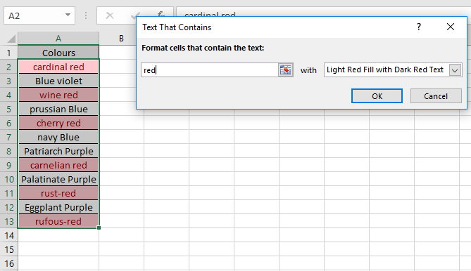
Here we have some of the shade colours of Blue, Purple & red.
We need to highlight all the cells which contains text red in the cell.
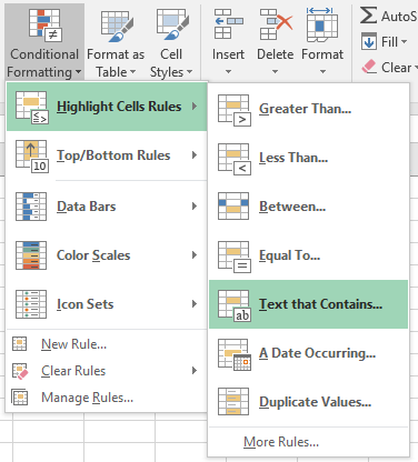
Go to Home > Conditional formatting > Highlight Cells Rules > Text that contains

Dialog box appears where we can add text rules.

As you can see from the above snapshot that only the cells which have text red in cells get highlighted.
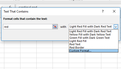
Select the type of formatting using Custom Format… option.

Select the colour format in the Format cells dialog box.

Sample box shows the type formatting selected.
Select Ok after confirming cell format

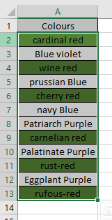
As you can see all the cells having text red are highlighted with Green Colour.
Hope you understood how to highlight cells that contain specific text with formulas in 2016. Explore more articles on Conditional formatting here. Please feel free to state your query or feedback in the comment box below. We will assist you.
Related Articles:
Conditional formatting based on another cell value in Excel
IF function and Conditional formatting in Excel
Perform Conditional Formatting with formula 2016
Conditional Formatting using VBA in Microsoft Excel
Popular Articles :
50 Excel Shortcut to Increase Your Productivity : Get faster at your task. These 50 shortcuts will make you work even faster on Excel.
How to use the VLOOKUP Function in Excel : This is one of the most used and popular functions of excel that is used to lookup value from different ranges and sheets.
How to use the COUNTIF function in Excel : Count values with conditions using this amazing function. You don't need to filter your data to count specific values. Countif function is essential to prepare your dashboard.
How to use the SUMIF Function in Excel : This is another dashboard essential function. This helps you sum up values on specific conditions.
The applications/code on this site are distributed as is and without warranties or liability. In no event shall the owner of the copyrights, or the authors of the applications/code be liable for any loss of profit, any problems or any damage resulting from the use or evaluation of the applications/code.