PivotTables in Excel 2010-Simplifying The Calculation

Pivot Tables are one of the most powerful features in excel. Even if you are a newbie, you can crunch large amounts of data into useful information. Pivot Table can help you make reports in minutes. Analyse your clean data easily and if the data is not clean, it can help you to clean your data. I don’t want to bore you, so let's jump into it and explore.

How To Create a Pivot Table

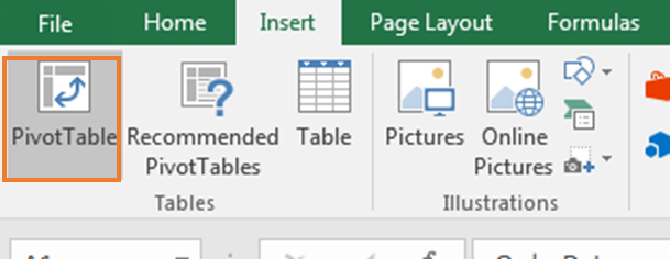
It's simple. Just select your data. Go to Insert. Click on the Pivot Table and it's done.

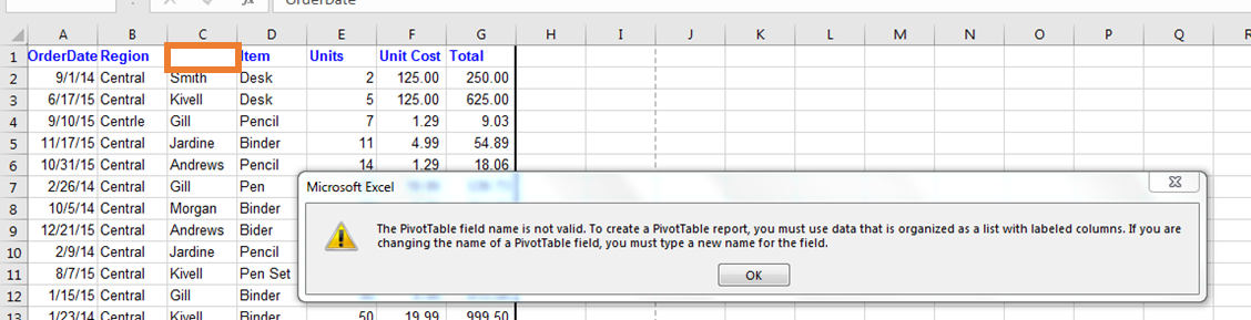
But wait. Before you create a pivot table, ensure that all columns have a heading.

If any column heading is left blank, the pivot table will not be created and will go through an error message.

Requirement 1: All columns should have a heading to get started with Pivot Tables in Excel

You should have your data organised with proper heading. Once you have it, you can insert the pivot table.

Insert the Pivot Table From Ribbon

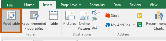
To insert a pivot table from the menu, follow these steps:

1. Select your data range
2. 
3. Go to the insert tab
4. 
5. Click on the Pivot Table icon
6. 
7. Create a Pivot Table option box will appear
8. 

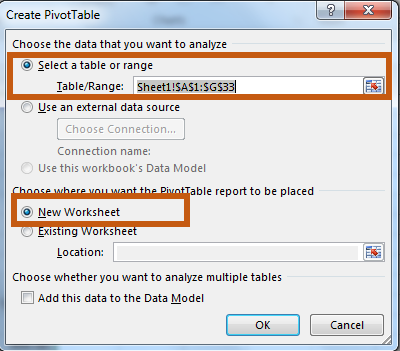
Here, you can see the data range that you selected. If you think that this is not the range you want to select, directly resize your range from here instead of going back and selecting data again.

Next, you can select where you want your pivot table. I recommend using the new worksheet but you can also use the current worksheet. Just define the location in the location box.

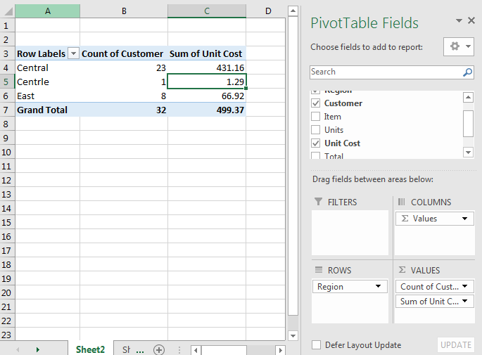
Now if you are done with the settings, hit the OK button. You will have your pivot table in a new sheet. Just select your fields for summaries. We will see how we create a summary of data using the pivot table but first let's get the basics clear. In this excel pivot table tutorial you will learn more than you expect.

Insert Pivot Table Shortcut (Alt > N > V)

This is a sequential keyboard shortcut to open the Create Pivot Table option box.

Hit the Alt button and release it. Hit N and release it. Hit V and release it.  Create a Pivot Table option box will open.

Now just follow the above procedure to create a pivot table in excel.

Insert Pivot Table Shortcut using Old Excel Shortcut (Alt > D > P)

One thing I like most about Microsoft Excel is that in every new version of Excel they introduce new features and but they don’t discard the old features (like MS did with win 8. It was pathetic). This allows the older user to work normally on new versions as they used to work on older versions.

If you sequentially press ALT, D and P on the keyboard, Excel will open to create a pivot table wizard.

Select the appropriate option. The selected option in the above screenshot will lead us to create a pivot table as we created before.

Hit Enter or click Next if you want to check your selected range.

Hit Enter again

Select a new worksheet or wherever you want your pivot table to Hit Enter. And it's done.

Excel pivot tables, first introduced in the market by Microsoft Excel 5 it is the perfect tool for all those who have trouble calculating, when you have a limited amount of data then calculators can do the job but when you have thousands of data to sum up then Excel pivot tables can be of great help to you. Pivot tables summarizes data in data visualization programs like spreadsheet, it can not only summarize but analyze, total and store the data in tables and can be used to build charts. Pivot tables are not exclusive to Microsoft a similar function called Data Pilot is found in OpenOffice.org software as well as Google Documents allows users to create basic pivot tables but nothing can be compared to Microsoft Excel pivot table.

Let’s take a deeper look on how pivot tables functions in Excel

First of all, type the data and click somewhere inside the data. Now go to the insert tag and click the pivot table button, excel will select all the data and asks you where to put the new pivot table. You can select it according to your choice then excel creates a place holder box where you have to tell excel to analyze the data for creating a pivot table. Then go to the pivot table field list which lists all the columns in the original data and drag any of them into any four regions underneath. Now excel would need to know the piece of information you want to summarize usually its numeric piece of information thus a simple pivot table is created. For more details you can subgroup the information by dragging any data from the field list to the row label. It is very simple to edit each piece of information. You can get more detailed summary by using more than one column. For grouping your data and using column label u can subdivide the columns and rows. When you split more than one piece of information into the row or column label excel gives you nifty boxes you can collapse some of these boxes to concentrate on the others.

New features in The Excel 2010 Pivot Table

• Multithreading has speeded up data retrieval and filtering in Pivot Tables making it faster.

• A new feature called Show Values is there .You have to right click the Pivot table and choose Show Values As. You will see many new options for different calculations and six new calculations that has been added to Excel 2010 Pivot Table

• You can combine items from different hierarchies using Named sets tools. While work with the same set of items excel 2010 can easily create and reuse logical grouping as a single object.

• You can modify values; recalculate new values even publish the modified data to the online analytical processing so that you can share it with other users. It includes a visual total by which the totals can be shown when one or more members are filtered.

If you have any further doubts about pivot tables you can use the help option in excel.

Hope this article about how to perform PivotTables in Excel 2010-Simplifying The Calculation in Excel is explanatory. Find more articles on Pivot table and editing table here. If you liked our blogs, share it with your friends on Facebook. And also you can follow us on Twitter and Facebook. We would love to hear from you, do let us know how we can improve, complement or innovate our work and make it better for you. Write us at info@exceltip.com

Related Articles:

subtotal grouped by dates in pivot table in Excel : find the subtotal of any field grouped by date values in pivot table using the GETPIVOTDATA function in Excel.

Pivot Table : Crunch your data numbers in a go using the PIVOT table tool in Excel.

Dynamic Pivot Table : Crunch your newly added data with old data numbers using the dynamic PIVOT table tool in Excel.

Show hide field header in the pivot table : Edit ( show / hide ) field header of the PIVOT table tool in Excel.

How to Refresh Pivot Charts : Refresh your PIVOT charts  in Excel to get the updated result without any problem.

Popular Articles:

How to use the IF Function in Excel : The IF statement in Excel checks the condition and returns a specific value if the condition is TRUE or returns another specific value if FALSE.

How to use the VLOOKUP Function in Excel : This is one of the most used and popular functions of excel that is used to lookup value from different ranges and sheets.

How to use the COUNTIF Function in Excel : Count values with conditions using this amazing function. You don't need to filter your data to count specific values. Countif function is essential to prepare your dashboard.

How to Use SUMIF Function in Excel : This is another dashboard essential function. This helps you sum up values on specific conditions.