

In this article, we will learn All about Check marks and Check boxes in Excel.
What is Check Mark and Check Box?
Check box is an object which is used to create a checklist for the data. Checkbox in excel is a dependent object which shows empty or ticked depending on the condition on the cell. Whereas Checkmark is a tick symbol used in Wingdings format. While writing some information or making a checklist, where elements are marked using a small tick mark. All the elements which are considered are marked with these tick marks. Many of us like to use the same in Excel. It makes data presentable and easy to understand.
Insert Check Marks Example :
All of these might be confusing to understand. Let's understand how to use the function using an example. Here First is by changing font style
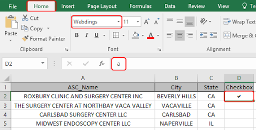
Go to Home > Select webdings in font style option and type alphabet a from the keyboard. You will see a checkmark on the selected cell.
The second method is by adding checkmark from symbols option
Go to Insert > Symbol

Symbol dialog box appears on your sheet.
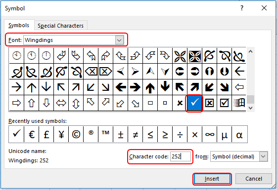
Select Wingdings in Font and type character code 252. Insert Checkmark.

As you can see check marks are added.
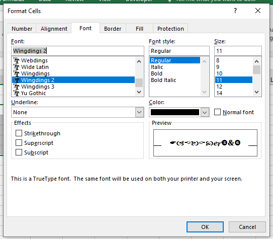
Check mark option is enabled in the format cell option. Use the Ctrl + 1 on the cell and select font option and then select wingdings 2. Wingdings 2 operate capital P as check mark in excel.
IF function excel tests the condition and returns value either it's True or False.
Syntax of IF function:
| = IF ( Logic_test , [value_if_true] , [Value_if_false] ) |
Logic test : operation to perform
The COUNTIF function of excel just counts the number of cells with a specific condition in a given range.
Syntax Of COUNTIF Statement
| = COUNTIF ( range , condition ) |
Range: it is simply the range in which you want to count values.
Condition: This is where we tell Excel what to count. It can be a specific Text (should be in “”), a number, a logical operator(=,><,>=,<=,<>) and wild card operators (*,?).
We will construct a formula to do our task. In logic_test argument we will use the countif function and for the value_if_True use the Capital P.
| = IF ( COUNTIF ( array , cell_value ), "P" , "" ) |
Let’s understand more about this function using it in an example.
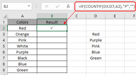
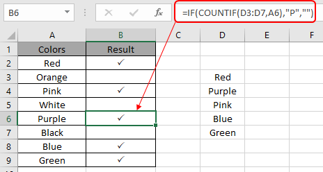
Here we have a list of colors data and and a list of colors which needed to be checked with colors data.

Here we need to use the formula to get the check mark symbol wherever required.
So we will use the formula to get the checkmark
| = IF ( COUNTIF ( D3:D7 , A2 ), "P" , "" ) |
Explanation:
COUNTIF will return 1 if the value is found or returns 0 if not. So the COUNTIF function works fine logic test for the IF function.
The IF function returns capital P if the value is 1 or else it returns an empty string if the value is 0.
Here the arguments to the function are given as cell reference.
Copy the formula to another cell using the Ctrl + D shortcut or drag down option in excel.
As you can see the check marks wherever required.
Insert Checkbox in Excel
To prepare the wedding checklist, we need an item list for wedding preparation, occasion, budget and checklist.
Items & Occasion:- Below are the list of Main Items and Occasions:-

Budget & %age of Items and Occasion need to spend: -Below is the list of Budget

Let’s continue with items:-
Step 1:-For every item, we have to define the sub items in which we will include each and everything. We have prepared the list for each item and occasion:-

Step 2:-
In front of list, enter the Estimated budget, Actual budget and Checklist:-
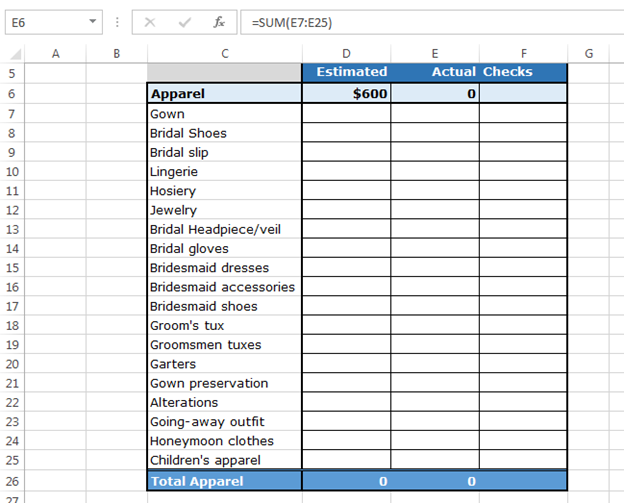
For example: -We have an Apparel list in range C6:C26.
Insert 3 columns: first for estimated budget, second for actual money spent and third for Checks
In cell D6, we will have the estimated budget which is linked to Sheet 2 where we have mentioned the estimated budget

Actual would be the sum of actual range =SUM(E7:E25)
Insert the check boxes by following below steps:-
Go to Developer tab > Controls group > Insert > Check box (form control)

After inserting the check box, right click with the mouse on check box

After inserting the check box, right click with the mouse on check box, pop up will appear

How to make a checklist?
Click on Edit text and delete the name of check box

Again, right Click on checkbox with the mouse and click on Format control from the pop-up
Format Control dialog box will appear
In Color and lines tab > Select the color for checkbox from fill color

In Color and lines tab > Select the color for checkbox

Once more, right click on the check boxes > Format Control > Control.

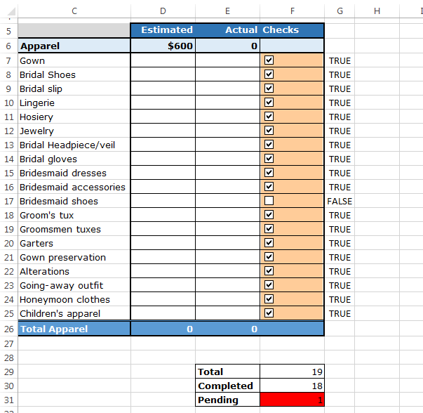
Link the cell with cell G7. When we check and uncheck the checkboxes, linked cell will change into true and false

Click on ok.

Now, copy the check box in the range and change the linked cell for every check boxes


According to the check boxes, we will return total no. of checkpoints completed and number of things that are left

Enter the formula for total nos:- =COUNTA(G7:G25)

Enter the formula for total Completed:- =COUNTIF(G7:G25,"True")

Note: When we check the check box then the linked cell will show true and, on uncheck, the result would be false.
To return pending no. we will subtract completed numbers from total numbers

This table will be helpful to track how many items are pending in the list.
Now, we will put the Conditional Formatting on pending cells, if the number of pending cells is zero, then cell color would be highlighted in green color; in case of greater than zero, it will be highlighted in red color.
Follow the steps below:-
Select the cell of Pending numbers
Go to Home tab > Conditional Formatting >New rule

New formatting rule dialog box will appear >Use a Formula to determine which cells to format >Enter the formula in format values box> =$F$31=0
Click on Format > Format cells dialog box will appear > Fill tab > Select green color

Click on OK

For second, follow the same process
Home Tab > Conditional Formatting >New formatting rule dialog box will appear > Use a Formula to determine which cells to format > Enter the formula in format values box > =$F$31>0
Click on Format > Fill Tab > Choose Red color > Click on ok > Click on ok

Note: - If you forgot any item, then this cell will be helpful to remind you that the items are still pending in the checklist.
Now, we will do the same thing for every checklist and then our wedding checklist will get prepared.
Here are all the observational notes using the formula in Excel.
Notes :
Hope this article about How to use the Check mark and Check box in Excel is explanatory. Find more articles on calculating values and related Excel formulas here. If you liked our blogs, share it with your friends on Facebook. And also you can follow us on Twitter and Facebook. We would love to hear from you, do let us know how we can improve, complement or innovate our work and make it better for you. Write to us at info@exceltip.com.
Related Articles :
How to use the Shortcut To Toggle Between Absolute and Relative References in Excel : F4 shortcut to convert absolute to relative reference and same shortcut use for vice versa in Excel.
How to use Shortcut Keys for Merge and Center in Excel : Use Alt and then follow h, m and c to Merge and centre cells in Excel.
How to Select Entire Column and Row Using Keyboard Shortcuts in Excel : Use Ctrl + Space to select whole column and Shift + Space to select whole row using keyboard shortcut in Excel
Paste Special Shortcut in Mac and Windows : In windows, the keyboard shortcut for paste special is Ctrl + Alt + V. Whereas in Mac, use Ctrl + COMMAND + V key combination to open the paste special dialog in Excel.
How to Insert Row Shortcut in Excel : Use Ctrl + Shift + = to open the Insert dialog box where you can insert row, column or cells in Excel.
Popular Articles :
50 Excel Shortcuts to Increase Your Productivity : Get faster at your tasks in Excel. These shortcuts will help you increase your work efficiency in Excel.
How to use the VLOOKUP Function in Excel : This is one of the most used and popular functions of excel that is used to lookup value from different ranges and sheets.
How to use the IF Function in Excel : The IF statement in Excel checks the condition and returns a specific value if the condition is TRUE or returns another specific value if FALSE.
How to use the SUMIF Function in Excel : This is another dashboard essential function. This helps you sum up values on specific conditions.
How to use the COUNTIF Function in Excel : Count values with conditions using this amazing function. You don't need to filter your data to count specific values. Countif function is essential to prepare your dashboard.
The applications/code on this site are distributed as is and without warranties or liability. In no event shall the owner of the copyrights, or the authors of the applications/code be liable for any loss of profit, any problems or any damage resulting from the use or evaluation of the applications/code.


