In our article, Count Cells That Contain Specific Text, we counted each cell that contains a specific text. In this article we will learn how to count cells that contains either this or that value. In other words, counting with OR logic.

You may think that you can use COUNTIF function two times and then add them up. But that is a wrong turn. You’ll know why.
Generic Formula
“This”: it is the first text you want count in the range. It can be any text.
“That”: it is the second text that you want to count in range. It can be any text.
Range: This is the range or array containing text in which you will count for your specific texts.
Let’s see an example:
Example:
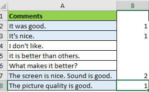
Here I have feedback comments in range A2 to A8. I want to count the number of comments containing “good” or “nice” words.

To count cells containing specific texts “good” or “nice” write this formula:

You can see that there are four comments that contain either “good” or “nice.”
How it works?
Let’s start from inside.
SEARCH("good",A2:A8): this part returns an array of #VALUE error and numbers, representing the position of found text. {8;#VALUE!;#VALUE!;#VALUE!;#VALUE!;30;24}
ISNUMBER(SEARCH("good",A2:A8)): this part of the formula checks each value in array return by SEARCH function, if it is a number or not, and returns an array of TRUE and FALSE. For this example, it returns {TRUE;FALSE;FALSE;FALSE;FALSE;TRUE;TRUE}.
ISNUMBER(SEARCH("nice",A2:A8)): this part of formula does the same, but this time it looks for “nice” word in cell and returns an array of the TRUE and FALSE base on cell contains the “nice.”
Next, we have added these arrays using + sign. It boolean values into 1 and 0 and adds them up. Internally it will look like this, {1;0;0;0;0;1;1}+{0;1;0;0;0;1;0}={1;1;0;0;0;2;1}.

You can see that comment in A7 has both texts “nice” and “good.” And it is double-counted here. We don’t want it. So we make another comparison for converting every number into True and False.
((ISNUMBER(SEARCH("good",A2:A8)) + ISNUMBER(SEARCH("nice",A2:A8)))>0): This part of formula converts the resultant array into TRUE and FALSE. If the value is greater than 0, it is TRUE else FALSE. Here it will be {TRUE;TRUE;FALSE;FALSE;FALSE;TRUE;TRUE}.
The number of TRUE in the array is the name of the string contain “good” or “nice” words.
SUMPRODUCT(--((ISNUMBER(SEARCH("good",A2:A8)) + ISNUMBER(SEARCH("nice",A2:A8)))>0))
Next we use -- negative symbols to convert them into numbers. And finally SUMPRODUCT sums up the array to return number of cells containing “good” or “nice”.
You can also use the SUM function, but then you’ll have to enter this formula as an array formula.
Why not use COUNTIFS?

Because of double counts.
If a cell contains both of the texts, then it will be counted twice, which is not correct in this scenario.
But if you want it to happen then use this formula,
It will return 5 in our example. I have explained it here.
Making Case Sensitive Count
The proposed solution counts the given text irrespective of the case of letters. If you want to count case sensitive matches, then replace SEARCH function with FIND function.
The FIND function is case sensitive function. It returns the position of found text.
So yeah guys, this how you can count the number of cells that contain either this text or that. You can also click on the function names in the formula to read about that function. I have understandably elaborated them.
Related Articles:
How to Check If Cell Contains Specific Text in Excel
How to Check a list of Texts In String in Excel
Get COUNTIFS Two Criteria Match in Excel
Get COUNTIFS With OR For Multiple Criteria in Excel
Popular Articles :
50 Excel Shortcut to Increase Your Productivity : Get faster at your task. These 50 shortcuts will make you work even faster on Excel.
How to use the VLOOKUP Function in Excel : This is one of the most used and popular functions of excel that is used to lookup value from different ranges and sheets.
How to use the COUNTIF function in Excel : Count values with conditions using this amazing function. You don't need to filter your data to count specific values. Countif function is essential to prepare your dashboard.
How to use the SUMIF Function in Excel : This is another dashboard essential function. This helps you sum up values on specific conditions.
The applications/code on this site are distributed as is and without warranties or liability. In no event shall the owner of the copyrights, or the authors of the applications/code be liable for any loss of profit, any problems or any damage resulting from the use or evaluation of the applications/code.