In this article, we will learn about how to partial match with VLOOKUP function in Excel.
VLOOKUP just searches for the row of a given value in the first column of a table and returns asked column’s value in that row.
Syntax:
Lookup_Value: The Value by which you want to search in the first column of Table Array.
Table_array: The Table in which you want to look up/search
col_index_number: The column number in Table Array from which you want to fetch results.
[range_lookup]: FALSE if you want to search for exact value, TRUE if you want an approximate Date match.
NOTE: VLOOKUP function looks up for the value in the first row of Table_array and extracts corresponding values only right of it
Let’s understand this function using it in an example.

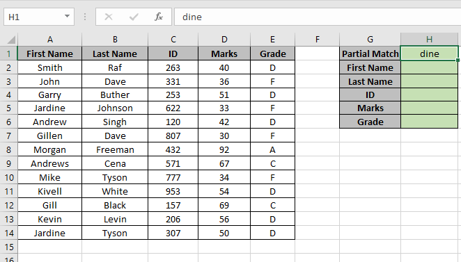
Here we have a Table named range A2:E14. And we need to find the partial match “dine” with the first name in the Table.
Use the formula:
“*dine*” : any first name that partially matches first name
Table : Table_array used define name on range A2:E14.
1 : look in the first column of the Table.
False : Accepts partial match.

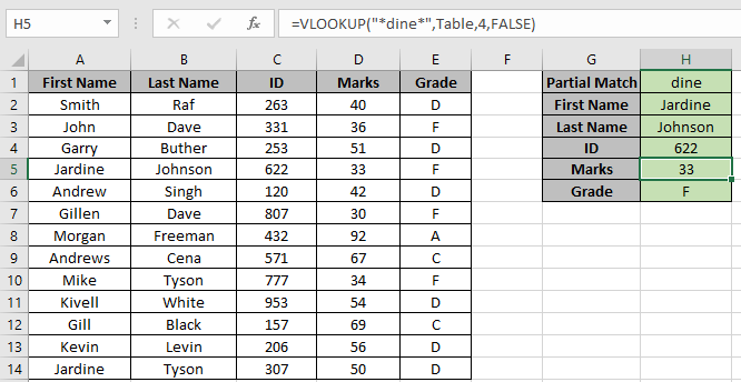
As you can see the first match with “dine” is “Jardine” and NOW we could find all the corresponding values of First Name Jardine.
Replace the col_index_number from 1 to 2, 3, 4 & 5 to get rest of the values.

As you can see we got all the values we need that matches our partial lookup value
Hope you understood how to use partial match with VLOOKUP function in Excel. Explore more articles on Excel LOOKUP function here. Please feel free to state your query or feedback for the above article.
Related Articles:
How to Get Position of First Partial Match
Popular Articles:
How to Use SUMIF Function in Excel
The applications/code on this site are distributed as is and without warranties or liability. In no event shall the owner of the copyrights, or the authors of the applications/code be liable for any loss of profit, any problems or any damage resulting from the use or evaluation of the applications/code.