

In this article, we will learn How to Color numbers based on the Value Result in Excel.
Scenario:
Formatting is only for the viewer's perception of the data. Whenever a number is entered in a cell in excel, The cell is in its general formatting. As default, the excel doesn't not assign any significance to the numbers that are being entered. But, for better presentation of data, the numbers need some different formatting. Hence, the range can be formatted as date or currency or accounting, percentage, fraction, etc. This function does not associate with the number, but just to the cell. Hence, if you enter a number 10/10/1986, the cell will format it as a date. But in the formula bar tab on the top of the worksheet, you will still see only 10/10/1986. A mere number such as ‘24’ can denote just about anything. But when you put a $ sign before it or a % sign after it, the entire value changes and so does the perception. These formatted numbers and signs do not interfere in any way with the calculations. That is why, in the formula bar, you will still see only the number.
Most of the time, Excel will suggest the formatting while the data is being typed in the cells. If it does not, then you can look for more options in the number format menu available in the home tab. If you do not find the required formatting in that list, you can create your own Excel custom format.
Home > Number > More number formats > Number tab > Custom. Here you will find existing number formats. This can be changed to create your own. The original from which the custom number format in Excel was made will still remain in the list, unchanged. If you no longer wish to use that custom format that you created, select it and click delete.
Conditional formatting is a whole different story. This is about formatting the individual cells in range affecting its colour, font, borders, etc. Where does the ‘condition’ in this come from? For example, you can set different conditions for the cell to change colour with. You can keep more than one condition for the same cell. For example, cell A1 containing a number less than 50 will be white; A2, 50 to 75 might be yellow and A3, 76 to 100 might be red. If you change the calculations or enter new data and the value of A3 drops down to 74, then it will automatically change colour from red to yellow.
Access Conditional formatting
Select a cell. Click on Home > Styles > conditional formatting. From the options you can create the conditions and choose different ways to exhibit it. You can highlight certain numbers that are being repetitive or are lesser than/greater than certain numbers, etc. Another option is to give a condition for highlighting % of a condition.
Example:
All of these might be confusing to understand. Let's understand how to use the function using an example. Here we have some values on the left side on which conditional formatting is being applied.
And on the right side we have some values on which the conditional formatting values are based upon.
We need to follow some steps
Select the cells A1 : C9.

Go to Home > Conditional Formatting > Highlight Cells Rules > Greater Than..

A dialog box will appear in front. Select the F3 cell in the first bow and select the formatting of the cells to Yellow Fill with Dark Yellow Text.

Click Ok.
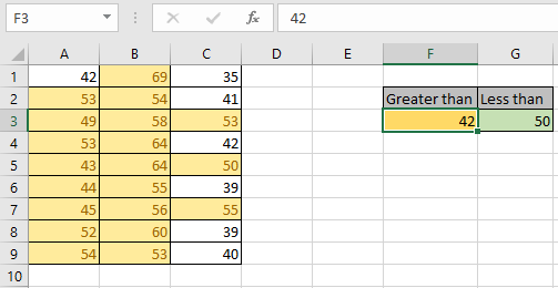
As you can see the format of all the values is changed wherever the condition matches.
You might also notice what happened to values between 42 & 50. Excel overwrites the first rule and gives preference to the last rule applied. If you wish to highlight the data with different colours. Make new rule in conditional formatting
Now we need to view the results based on another cell value. For that go through the same process. Starting from Selecting the range

Go to Home > Conditional Formatting > Highlight Cells Rules > Less Than..
A dialog box will appear in front

Select the G3 cell in the first bow and select the formatting of the cells to Green Fill with Dark Green Text as shown in the snapshot below.

Click Ok.
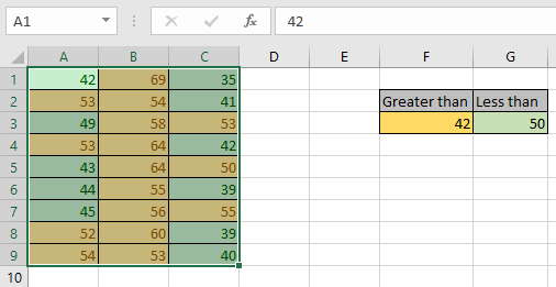
As you can see the new format of values is changed using Conditional formatting based on cell values.
Changing the values in the cell changes result.

As you can see we changed the value in G3 cell from 50 to
40 and can view the updated results.
Using Formula in Conditional formatting:
You can perform the above stated task using formulas in conditional formatting. Learning this will enhance your excel skills.
Here we have data on sales done by different dealerships in months of different years. I want to highlight sales in 2019 that are greater than sales in 2018.

To do so, follow these steps.
Select range D2:D12 (Sales of 2019)
Go to Home > Conditional Formatting > New Rule. Here, select "Use a formula to determine which cell to format"
In the formula box, write this excel formatting formula.
| =$D2>$C2 |
Select the formatting of the cell if the condition is true. I have selected a green fill.

Hit the OK button.
And it's done. All the values in sales 2019 that are greater than the sales in 2018 are highlighted with green fill.

Explanation
It's easy. First, we select the range on which we want the formula to apply. Next, we use a formula to determine which cell to format in the selected range. The formula is $D2>$C2. Here we have locked columns and allowed rows to change. This is called half absolute referencing. Now, D2 is compared with C2, since D2 is greater than C2, D2 is filled with green colour. Same happens with each cell.
If you wanted to highlight months instead of sales in 2019, you can directly change "formula applies to" to the range A2:A12.
Select any cell in D2:D12. Go to conditional formatting. Click on "Manage Rules".
Change the range in the "Applies to" box to A2:A12.

Hit the OK button.

You can see that formatting is applied to the mentioned reference. Similarly, you can format any range based on any column in excel. The column can be on a different sheet too. You just need to mention the range. You can also mention the non-connected ranges. Just use a comma between ranges in the "applied to" section.

As you can see the results in the snapshot above.
Here are all the observational notes using the formula in Excel.
Notes :
Hope this article about How to How to Color numbers based on the Value Result in Excel is explanatory. Find more articles on calculating values and related Excel formulas here. If you liked our blogs, share them with your friends on Facebook. And also you can follow us on Twitter and Facebook. We would love to hear from you, do let us know how we can improve, complement or innovate our work and make it better for you. Write to us at info@exceltip.com.
Related Articles :
Find the partial match number from data in Excel : find the substring matching cell values using the formula in Excel
How to Highlight cells that contain specific text in Excel : Highlight cells based on the formula to find the specific text value within the cell in Excel.
Conditional formatting based on another cell value in Excel : format cells in Excel based on the condition of another cell using some criteria.
IF function and Conditional formatting in Excel : How to use IF condition in conditional formatting with formula in excel.
Perform Conditional Formatting with formula 2016 : Learn all default features of Conditional formatting in Excel
Conditional Formatting using VBA in Microsoft Excel : Highlight cells in the VBA based on the code in Excel.
Popular Articles :
50 Excel Shortcuts to Increase Your Productivity : Get faster at your tasks in Excel. These shortcuts will help you increase your work efficiency in Excel.
How to use the VLOOKUP Function in Excel : This is one of the most used and popular functions of excel that is used to lookup value from different ranges and sheets.
How to use the IF Function in Excel : The IF statement in Excel checks the condition and returns a specific value if the condition is TRUE or returns another specific value if FALSE.
How to use the SUMIF Function in Excel : This is another dashboard essential function. This helps you sum up values on specific conditions.
How to use the COUNTIF Function in Excel : Count values with conditions using this amazing function. You don't need to filter your data to count specific values. Countif function is essential to prepare your dashboard.
The applications/code on this site are distributed as is and without warranties or liability. In no event shall the owner of the copyrights, or the authors of the applications/code be liable for any loss of profit, any problems or any damage resulting from the use or evaluation of the applications/code.


Gayle, clieck on the cell that has the hyperlink (red and underlined) , it will go to the web site . GO back to that cell. Then on the menu bar , go to Insert, Hyperlink. In the window that opens up , go to the bottom left where there is an option "Remove Link", select that. Your cell will not have that hyperlink anymore.
Thanks, but we already tried that and it didnt work. Eversince she put the email address into the column, everything now in that column turns red and is highlighted as if it were a link.
"Select the cell, click on Format - Cells.
Change it to General or whatever format you prefer.
Alternatively, use the format painter icon to copy the format of another phone number that is already how you want it to look. "
A friend of mine is working on a spreadsheet. She is inputting contact information and in one particular column she is adding phone numbers. In that column, she added an email address and it automatically turned into a link (it was underlined and the type turned red). Now when she attempts to type a phone number in that same column, different cell, it turns red and is underlined. What is happening here and how can she eliminate whatever formatting is occurring????
Gayle, click on the cell that has the hyperlink (red and underlined) , it will go to the web site . GO back to that cell. Then on the menu bar , go to Insert, Hyperlink. In the window that opens up , go to the bottom left where there is an option "Remove Link", select that. Your cell will not have that hyperlink anymore.
Gayle, clieck on the cell that has the hyperlink (red and underlined) , it will go to the web site . GO back to that cell. Then on the menu bar , go to Insert, Hyperlink. In the window that opens up , go to the bottom left where there is an option "Remove Link", select that. Your cell will not have that hyperlink anymore.
"Hey Alan,
Thanks, but we already tried that and it didnt work. Eversince she put the email address into the column, everything now in that column turns red and is highlighted as if it were a link.
Gayle"
"Hi Gayle,
Select the cell, click on Format - Cells.
Change it to General or whatever format you prefer.
Alternatively, use the format painter icon to copy the format of another phone number that is already how you want it to look.
HTH,
Alan."
"Hi,
A friend of mine is working on a spreadsheet. She is inputting contact information and in one particular column she is adding phone numbers. In that column, she added an email address and it automatically turned into a link (it was underlined and the type turned red). Now when she attempts to type a phone number in that same column, different cell, it turns red and is underlined. What is happening here and how can she eliminate whatever formatting is occurring????
Thanks!"