
In this article, we will learn How to Coloring One Record in Each Group in a Range in Excel.
Scenario:
Sometimes given a list of values we need to highlight only first output or unique values. For example if we need to highlight the entries where a customer once transacted in a store. If an entry is repeated, then it shouldn't be highlighted. Excel provides us with a conditional formatting tool and some formula logic. Using Conditional formatting over cells and then adding values on it. So we need a formula for the data which highlights cells only matching one record matching values.
How to solve the problem?
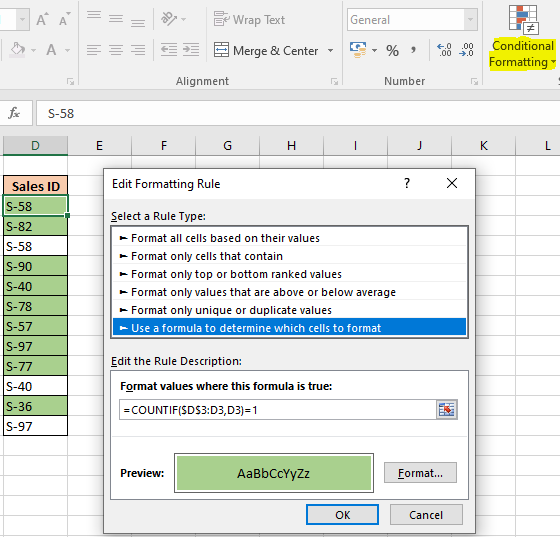
For this we will be using the Conditional formatting obviously and COUNTIF function. This formula is derived using Expanding References. Where we first input formula to the first cell and then copy and paste the formatting (with formula) on to the required range. This formula only highlights the first record or the unique records.
Generic formula:
| =COUNTIF($D$3:D3,D3)=1 |
cell : first cell of the range (we don't need to specify the last cell, expanding references will take care of it)
=1 : equals to operator to match criteria (first record)
Example :
All of these might be confusing to understand. Let's understand this formula by running it on an example. Here we have data with entries of the staff in an office. There are multiple entries of some staff members. We need to highlight the first entry. Follow the steps:
Use the formula for matching value less than 50000.
| =COUNTIF($D$3:D3,D3)=1 |
Explanation:

Select the format as you require, it offers many different types of formatting. We selected to color fill the record or cell as shown above. Click OK
Now copy the cell and paste till the range either using Ctrl + C (to copy) and Ctrl + V (to paste) or select the cell and drag it to right or bottom as you require to apply.
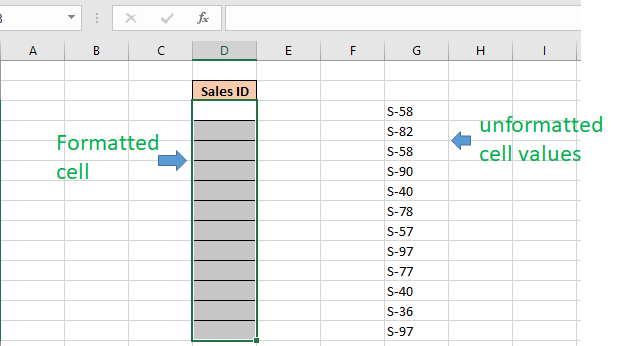
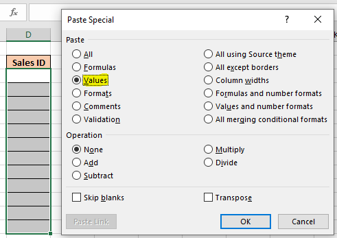
Copy the unformatted cell values and paste only the values using (Ctrl + Alt + V) or using paste special (opens using the right mouse button.
Click Ok and you can see, Conditional formatting does all the highlighting for you.

Here are all the observational notes regarding using the formula.
Notes:
Hope you understood How to highlight or Color One Record in Each Group in a Range in Excel. Explore more articles on Excel highlighting cells with formulas here. If you liked our blogs, share it with your friends on Facebook. And also you can follow us on Twitter and Facebook. We would love to hear from you, do let us know how we can improve, complement or innovate our work and make it better for you. Write to us at info@exceltip.com.
Related Articles:
Expanding References in Excel : The ranges that expand when copied in the below cells or to right cells are called expanding references. Where do we need expanding references? Well, there were many scenarios.
Find the partial match number from data in Excel : find the substring matching cell values using the formula in Excel.
How to Highlight cells that contain specific text in Excel : Highlight cells based on the formula to find the specific text value within the cell in Excel.
Conditional formatting based on another cell value in Excel : format cells in Excel based on the condition of another cell using some criteria in Excel.
IF function and Conditional formatting in Excel : How to use IF condition in conditional formatting with formula in Excel.
Perform Conditional Formatting with formula 2016 : Learn all default features of Conditional formatting in Excel.
Conditional Formatting using VBA in Microsoft Excel : Highlight cells in the VBA based on the code in Excel.
Popular Articles :
50 Excel Shortcut to Increase Your Productivity : Get faster at your task. These 50 shortcuts will make you work even faster on Excel.
How to use the VLOOKUP Function in Excel : This is one of the most used and popular functions of excel that is used to lookup value from different ranges and sheets.
How to use the COUNTIF function in Excel : Count values with conditions using this amazing function. You don't need to filter your data to count specific values. Countif function is essential to prepare your dashboard.
How to use the SUMIF Function in Excel : This is another dashboard essential function. This helps you sum up values on specific conditions.
The applications/code on this site are distributed as is and without warranties or liability. In no event shall the owner of the copyrights, or the authors of the applications/code be liable for any loss of profit, any problems or any damage resulting from the use or evaluation of the applications/code.


"Was trying to find a way to colour cells automatically; never even knew that this function existed- was lucky to have found this site on the web.
Just what I needed "
Lets say I have a set of numbers in cel A1 and I have a description in cell G1. If I type the words test in G1, I want A1 to become a color. How would I do this?
"Probably the reason is that things are not as 'obvious' as they may appear.
I suggest you take your nested IFs and pull them out into separate cells (take them to a calculation sheet if necessary).
It is generally bad form to nest IF statements to deep anyway, since they become very difficult to 'read' and de-bug (as you have discovered).
Once you have done that, you will find that one specific logical test is not behaving as you expect. If you still can't work it out, post that specific test / data back here, and hopefully we can help. "
I would like to write a formula that identifies only the first cell in a range of values that is greater than zero.
can anyone help me in this. I have a range of cells with numbers. I use count function to count the range. But I want a cell to be counted or added to count function ONLY when I FILL COLOR to a particular cell. is this possible?
I want a function through which I can set or change the format of a cell entry. Although I can do it through "conditional formatting" option, but it permits only three conditions. I want more options.
"And in step 5:
=COUNTIF($A$2:$A2,$A2)=1"
If you have more than one column of data, then in Step 2, first press CTRL+SHIFT+RIGHT ARROW to select all the columns of data, and then press CTRL+SHIFT+DOWN ARROW to select all the rows of data. Then continue with the remaining steps.
Only the perticular cell is coloured , how can I colour the enrire row of a unique record.
"Was trying to find a way to colour cells automatically; never even knew that this function existed- was lucky to have found this site on the web.
Just what I needed "
"Just use the conditional formatting feature (select the 'FORMULA IS' option).
The help facility explains it in detail quite neatly. "
"Lets say I have a set of numbers in cel A1 and I have a description in cell G1. If I type the words test in G1, I want A1 to become a color. How would I do this?
"
"Probably the reason is that things are not as 'obvious' as they may appear.
I suggest you take your nested IFs and pull them out into separate cells (take them to a calculation sheet if necessary).
It is generally bad form to nest IF statements to deep anyway, since they become very difficult to 'read' and de-bug (as you have discovered).
Once you have done that, you will find that one specific logical test is not behaving as you expect. If you still can't work it out, post that specific test / data back here, and hopefully we can help. "
"I am using a nested (if(and( formula that is giving me a value of ""false"". However, the conditions are clearly met by the last if/and statement and not met by any of the previous if/and statements of which there are five in total. What could be the source of this problem?
Thank you very much for your help. "
"Try this:
{=INDEX(Range,MATCH(TRUE,(Range)>0,0))}
This assumes, at least implicitly, that 'Range' is one-dimensional.
This is an array formula, so enter it without the curly brackets, using Shift-Ctrl-Enter. "
"""If I want that the entire row to be colored whenever a cell has a certain value, say if cell has the value ""A"", then the entire row should be colored red, and so on. How can I achieve this task.""
I am also searching for this answer. Any help for this novice would be appreciated..."
can anyone help me in this. I have a range of cells with numbers. I use count function to count the range. But I want a cell to be counted or added to count function ONLY when I FILL COLOR to a particular cell. is this possible?
If I want that the entire row to be colored whenever a cell has a certain value, say if cell has the value "A", then the entire row should be colored red, and so on. How can I achieve this task.
I want a function through which I can set or change the format of a cell entry. Although I can do it through "conditional formatting" option, but it permits only three conditions. I want more options.
"And in step 5:
=COUNTIF($A$2:$A2,$A2)=1"
If you have more than one column of data, then in Step 2, first press CTRL+SHIFT+RIGHT ARROW to select all the columns of data, and then press CTRL+SHIFT+DOWN ARROW to select all the rows of data. Then continue with the remaining steps.
Only the perticular cell is coloured , how can I colour the enrire row of a unique record.