
In this article, we will learn Introduction to Advance Filter in Excel.
What is Advanced Filter ?
Advance Filter is the most powerful feature of Excel. The advanced filtering feature in Excel allows you to quickly copy unique information from one data list to another. It allows the person to quickly remove duplicates, extract records that meet certain criteria. It works great when we use wildcards, within 2 date criteria.
Filtering is a simple, however, amazing & powerful way to analyze data. Advance filter are quite easy to use. Here's how you can use Excel's advanced filtering capabilities.
Scenario:
In simple words, while working with table values, sometimes we need to count, sum, product or average of the values having already applied filter option. Example if we need to get the count of a certain IDs where the ID data has applied filter on. Criteria on data is applied using the filter option.
How to solve a filtered problem using a function ?
For this article we will be required to use the SUBTOTAL function. Now we will make a formula out of the function. Here we are given some values in a range and specific text value as criteria. We need to count the values where the formula includes all the values which ends with the given text or pattern
Generic formula:-
| = SUBTOTAL ( fun_num, range ) |
fun_num : number, num corresponding to the operation
range : range where operation is to apply.
Example:
All of these might be confusing to understand. So, let's test this formula via running it on the example shown below.
Here we have the order import data. And we have applied criteria to Region, only the East region is filtered.
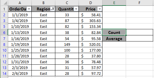
Here to find the count of filtered values. Choose the right argument as fun_num. Fun_num is the operation you want to apply. Here to count the cells we use COUNTA operation, num as 3.
Use the formula:
| = SUBTOTAL ( 3, B2:B14) |

As you can see the total rows which are visible comes out to be 11. Now we will use one more example to extract the Average of the quantity which are visible or filtered.
Use the formula:
| = SUBTOTAL ( 1 , C2:C14 ) |

As you can see the average order quantity received from the East region comes out to be approx 60. You can use different operations like average, count, max, min, product, standard deviation, sum or variation as per the required results on filtered data.
Let’s understand this with an example.
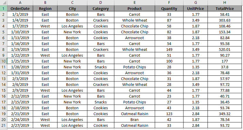
Here we have a data set.
Now we need to delete the rows with City : Boston
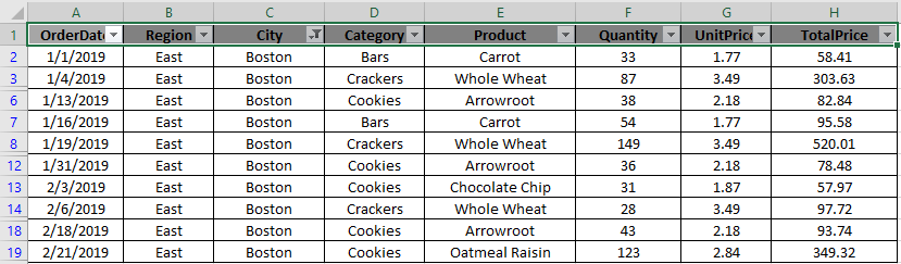
As you can see filtered Rows with City:Boston
Now I will select these rows which are to be deleted.
Go to Home > Find & Select > Go To Special

Go To Special dialog box appears

Select Visible cells only > OK
You will see the selected region as shown below. Right click on any selected cell > Select Delete Row

It shows a warning as shown below
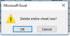
Click Ok.

As you can see selected rows are deleted. To view other cells. To view other cells, Double click on the red part shown in the left in the snapshot.

You will get your desired output as shown below in the table.

This is a very useful function while editing data in your worksheet.
Here are some observational notes shown below.
Notes:
Hope this article about Introduction to Advance Filter in Excel is explanatory. Find more articles on sort and Filter values and related Excel formulas here. If you liked our blogs, share it with your friends on Facebook. And also you can follow us on Twitter and Facebook. We would love to hear from you, do let us know how we can improve, complement or innovate our work and make it better for you. Write to us at info@exceltip.com.
Related Articles
How to use the SUBTOTAL function in Excel: Returns the SUM, COUNT, AVERAGE, STDEV or PRODUCT on applied filtered data in Excel.
COUNTIFS with Dynamic Criteria Range : Count cells dependent on other cell values in Excel.
COUNTIFS Two Criteria Match : Count cells matching two different criteria on list in excel.
COUNTIFS With OR For Multiple Criteria : Count cells having multiple criteria match using the OR function.
The COUNTIFS Function in Excel : Count cells dependent on other cell values.
How to Use Countif in VBA in Microsoft Excel : Count cells using Visual Basic for Applications code.
How to use wildcards in excel : Count cells matching phrases using the wildcards in excel
Popular Articles :
How to use the IF Function in Excel : The IF statement in Excel checks the condition and returns a specific value if the condition is TRUE or returns another specific value if FALSE.
How to use the VLOOKUP Function in Excel : This is one of the most used and popular functions of excel that is used to lookup value from different ranges and sheets.
How to Use SUMIF Function in Excel : This is another dashboard essential function. This helps you sum up values on specific conditions.
How to use the COUNTIF Function in Excel : Count values with conditions using this amazing function. You don't need to filter your data to count specific values. Countif function is essential to prepare your dashboard.
The applications/code on this site are distributed as is and without warranties or liability. In no event shall the owner of the copyrights, or the authors of the applications/code be liable for any loss of profit, any problems or any damage resulting from the use or evaluation of the applications/code.


Good
Advance Filters are very useful, but it's a big call to say "Advance Filter is the most powerful feature of Excel." I doubt you'll find many agreeing with you that they're more powerful than Pivot Tables, or the new PowerPivot in 2013.
Completely agree with you but do you have idea how many users use 2013???
I wonder they will be many who are still using 2007 or 2010. So this is good for them and specially for beginners.
Thanks a lot
Am I just an idiot? I cannot replicate this to save my life. Nothing is filtering after I click OK.
Are you setting up the Criteria Range? The post doesn't explain it well. Where it says "In Criteria range; select the criteria range as I1:N2", see that it shows Susan in the appropriate cell (the 5th column over from the beginning of the range, just as manager in the data is the 5th column of that range). The post doesn't really explain doing this, just shows an image.
Hi Slightly Less Confused,
You need to download the excel file & follow below steps:
• In Excel file you will find Raw Data sheet.
• Copy the header range A1:F1 & paste to range I1:N1
• In Manager column i.e. in cell M2 type "Susan"
• Then press shortcut keys ALT + A + Q & follow the steps mention in the book.
I follow the same & got the filter data.
@AfroDaby: Hope this will help you.
Regards,
Ashish
This is great!
Great
thanks