
I missed to pay my Cell Phone, Internet bill on time. In case you have came across with this problem then this article is for you.
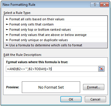
In this example, we will use AND, TODAY functions in Conditional Formatting.
Let us take an example:
We have bills in column A & due date in column B.

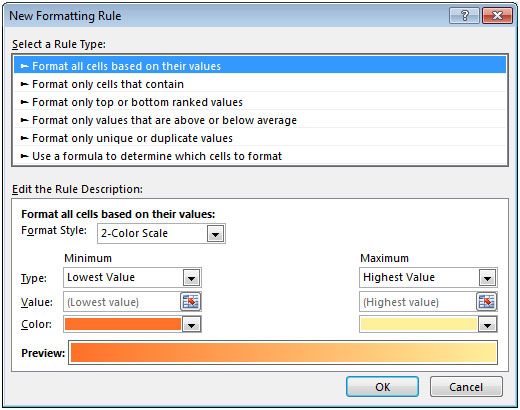
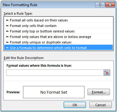
Select New Rule

Note: Today’s date in above formula is 27-Jan-15
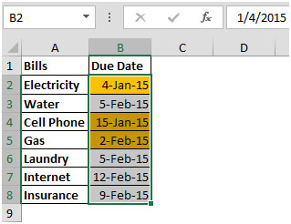
In this way you can highlight the due dates cells which are expired & 7 days left for passing the due date.
With above example, you can create various notifications or alert depending on the requirement.
The applications/code on this site are distributed as is and without warranties or liability. In no event shall the owner of the copyrights, or the authors of the applications/code be liable for any loss of profit, any problems or any damage resulting from the use or evaluation of the applications/code.


Hello, and thank you for your page. I have followed the process to the T, but it doesn't highlight anything. Any suggestions?
This one remain when open excel or open system
Pls clarify
Tq