
What is Intercept?
Intercept is a point on Y-axis where the line crosses. Or, we can say that it is the value of y when x is 0.
How to find the y-intercept of a function? The formula for Intercept for a simple line connecting two points on the line is:
b (intercept) = y- mx
where b is Intercept. y is y co-ordinate and x is x co-ordinate. m is the Slope of a line.
When we have multiple xs and ys (like most of the time). At that time we take the average of each intercept to get the y-intercept of the regression.
b=AVERAGE(yi-mxi)
How to Calculate Intercept in Excel
To calculate Intercept in Excel we do not need to do much hassle. Excel provides the INTERCEPT function that calculates the y-intercept of the line or regression. The INTERCEPT function is a statistical function of excel widely used in statistical analysis in excel.
Syntax of the INTERCEPT function
| =INTERCEPT(known_ys, known_xs) |
known_ys: the array of y values.
known_xs: the array of x values.
Note that the number of xs and ys should be the same.
I will calculate the y-intercept manually at the end of the article so that we can understand how it is being calculated.
Calculate the y-intercept in Excel
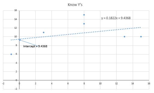
Let's have an example to understand how we can easily calculate the y and x-intercept in excel. Here I have a sample data of know ys and xs.
 So to calculate y-intercept we use the INTERCEPT function.
| =INTERCEPT(B2:B7,A2:A7) |
Here known ys are in range B2:B7 and known xs are in range A2:A7. This returns the intercept as 9.436802974. If you want to calculate x-intercept then just reverse the order in the formula i.e. =INTERCEPT(A2:A7,B2:B7). It will return 0.110320285.

Now the question arrives:
How does it work?
To understand how we get our intercept of the function, we need to calculate the intercept manually. It is quite easy. Let's see.
As I mentioned at the beginning of the article, the mathematical formula for y-intercept is
b=y-mx
Now follow these steps.
| =SLOPE(B2:B7,A2:A7) |
| =B2-($A$10*B2) |
the formula is equivalent to y-mx. Now we have an intercept for each point.
Now we just need to get the average or mean of these intercepts to get the intercept of the regression. Write this formula in A12.
| =AVERAGE(C2:C7) |

It returns 9.436802974. This is equal to the value returned by the INTERCEPT function.
You can see how we get our intercept manually. All this task is done using the INTERCEPT function in the background.
Now we know how we can calculate intercept in excel for statistical analysis. In regression analysis, we use the intercept of the equation. You can see the practical use of INTERCEPT here.
I hope I was explanatory enough. Let me know if this was helpful. If you have any doubts regarding the calculation of intercept in excel or any other excel topic, mention it in the comment section below.
Related Data:
How to Use STDEV Function in Excel
How To Calculate MODE
How To Calculate Mean
How to Create Standard Deviation Graph
Descriptive Statistics in Microsoft Excel 2016
How to Use Excel NORMDIST Function
Popular Articles:
The applications/code on this site are distributed as is and without warranties or liability. In no event shall the owner of the copyrights, or the authors of the applications/code be liable for any loss of profit, any problems or any damage resulting from the use or evaluation of the applications/code.


