

In this article, we will learn How to LOOKUP value between two numbers in Excel.
Scenario:
It's easy to look up a value with one criteria in a table. We can simply use VLOOKUP. But what could we do if have that multiple column criteria to match in your data and need to lookup in multiple columns to match a value. Let's learn how this problem can be solved using different lookup versions of excel
LOOKUP value between two numbers
Using VLOOKUP formula
In VLOOKUP approximate match, if a value is not found then the last value that is less than the lookup value is matched and the value from the given column index is returned.
Generic formula to LOOKUP value between two numbers:
| = VLOOKUP (value, table, lookup_col , 1 ) |
And one more thing about Vlookup is it looks for the value in the column and if it doesn’t find the value in the column array then it matches and returns the value that is less than that value in the table array.
Note : VLOOKUP by default does an approximate match, if we omit the range lookup variable. An approximate match is useful when you want to do an approximate match and when you have your table array sorted in ascending order.
Using INDEX and MATCH formula
The INDEX and MATCH formula does the same work as above but with different syntax. But if you should only choose the one with which functions you are comfortable with
Generic Formula to LOOKUP value between two numbers
| =INDEX(lookup_range,MATCH(1,INDEX((criteria1=range1)*(criteria2=range2),0,1),0)) |
lookup_range: the range from which you want to retrieve value.
Criteria1, Criteria2, Criteria N: These are the criteria you want to match in range1, range2 and Range N. You can have upto 270 criteria - range pairs.
Range1, range2, rangeN : These are the ranges in which you will match your respective criteria.
Example :
All of these might be confusing to understand. Let's understand how to use the function using an example. Here we have Student ID and their respective marks in a test. Now we had to get the grades for each student via looking up in the grade system table.

To do so, we will use an attribute of the VLOOKUP function which is if the VLOOKUP function doesn't find the exact match it looks for the approx match in the table only and only if the last argument of the function is either TRUE or 1.
The marks / score table must be ascending order
Use the formula:
| = VLOOKUP ( B2 , table , 2 , 1 ) |
How does it work?
The Vlookup function looks up the value 40 in the marks column and returns the corresponding value, if matched. If it does not match then the function looks for the lesser value than the lookup value (i.e 40) and returns its result.
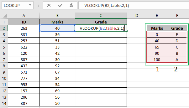
Here the table_array is named range as table in formula and B2 is given as cell reference.

As you can see we got the grade for the first student. Now to get all other Grades, we will use shortcut Ctrl + D or use drag down cell option in excel.

Here are all the Grades of the class using the VLOOKUP function.
LOOKUP value between two numbers on Employee table
We have a table that contains the details of all the employees in an organization on a separate sheet. The first column contains the ID of these employees. I have named this table as emp_data.

Now my search sheet needs to fetch the employee's information whose ID is written in cell B3. I have named B3 as ID.

For ease of understanding, all the column heading are in exactly the same order as the emp_data table.
Now write the below formula in cell C3 to retrieve the zone of the employee ID written in B3.
| =VLOOKUP(ID,Emp_Data,2,0) |
This will return the zone of the employee Id 1-1830456593 because column number 2 in the database contains the zone of employees.
Copy this formula in the rest of the cells and change the column number in the formula to get all the information of employees.
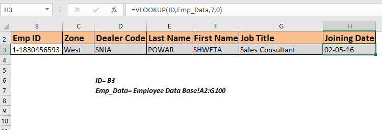
You can see all the information related to the mentioned ID in Cell B3. Whichever id you write in Cell B3, all the information will be fetched without making any change in the formula.
How does this work?
There's nothing tricky. We are simply using the VLOOKUP function to lookup ID and then fetch the mentioned column. Practice VLOOKUP using such data to understand the VLOOKUP more.
In the above example, we had all the columns organized in the same order but there will be times when you'll have a database that will have hundreds of columns. In such cases, this method of retrieving employee information won't be good. It will be better if the formula can look at the column heading and fetch data from that column from the employee table.
So to retrieve value from the table using column heading we will use a 2-way lookup method or say dynamic column VLOOKUP.
Use this formula in cell C3 and copy in the rest cells. You don't need to change anything in the formula, everything will be fetched from thd emp_data.
| =VLOOKUP(ID,Emp_Data,MATCH(C2,Emp_Data_Headers,0),0) |

This formula simply retrieves all the information from matched columns. You can jumble the headers in the report, this won't make any difference. Whichever the heading is written in the cell above, the respective data contains.
How does this work?
This is simply a dynamic VLOOKUP. You can read about it here. If I'll explain it here, it will become a too large article.
It may happen that you don't remember the whole ID of an employee, but you still want to retrieve the information of some ID. In such cases partial match VLOOKUP is the best solution.
For example, If I know that some id contains 2345 but I don't know the whole Id. If I enter this number in Cell C3, the output will be like.

We get nothing. Since nothing matches 2345 in the table. Modify the above formula like this.
| =VLOOKUP("*"&ID&"*",Emp_Data,MATCH(C2,Emp_Data_Headers,0),0) |
Copy this in the entire row. And now you have the information of the first employee that contains this number.

Please note that we will get the first ID that contains the matched number in the Emp Id column. If any other ID contains the same number, this formula will not retrieve that employee's information.
If you want to get all the employee ids that contain the same number use the formula that looks up all the matched values.
Using INDEX and MATCH formula
Here we have a data table. I want to pull the Name of the customer using Date of Booking, Builder and Area. So here I have three criteria and one lookup range.
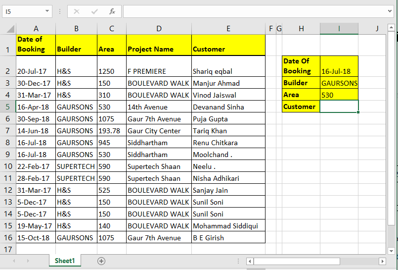
Write this formula in cell I4 hit enter.
| =INDEX(E2:E16,MATCH(1,INDEX((I1=A2:A16)*(I2=B2:B16)*(I3=C2:C16),0,1),0)) |

How it works:
We already know how INDEX and MATCH function work in EXCEL, so I am not going to explain that here. We will talk about the trick we used here.
(I1=A2:A16)*(I2=B2:B16)*(I3=C2:C16): The main part is this. Each part of this statement returns an array of true false.
When boolean values are multiplied they return an array of 0 and 1. Multiplication works as an AND operator. Hense when all value are true only then it returns 1 else 0
(I1=A2:A16)*(I2=B2:B16)*(I3=C2:C16) This altogether will return
| {FALSE;FALSE;FALSE;FALSE;FALSE;FALSE;TRUE;TRUE;FALSE;FALSE;FALSE;FALSE;FALSE;FALSE;FALSE}*
{FALSE;FALSE;FALSE;TRUE;TRUE;TRUE;TRUE;TRUE;FALSE;FALSE;FALSE;FALSE;FALSE;FALSE;TRUE}* {FALSE;FALSE;FALSE;TRUE;FALSE;FALSE;FALSE;TRUE;FALSE;FALSE;FALSE;FALSE;FALSE;FALSE;FALSE} |
Which will translate into
| {0;0;0;0;0;0;0;1;0;0;0;0;0;0;0} |
INDEX((I1=A2:A16)*(I2=B2:B16)*(I3=C2:C16),0,1): INDEX Function will return the same array ({0;0;0;0;0;0;0;1;0;0;0;0;0;0;0}) to MATCH function as lookup array.
MATCH(1,INDEX((I1=A2:A16)*(I2=B2:B16)*(I3=C2:C16),0,1): MATCH function will look for 1 in array {0;0;0;0;0;0;0;1;0;0;0;0;0;0;0}. And will return the index number of first 1 found in the array. Which is 8 here.
INDEX(E2:E16,MATCH(1,INDEX((I1=A2:A16)*(I2=B2:B16)*(I3=C2:C16),0,1),0)): Finally, INDEX will return the value from the given range (E2:E16) at found index (8).
Here are all the observational notes using the formula in Excel
Notes :
Hope this article about How to LOOKUP value between two numbers in Excel is explanatory. Find more articles on calculating values and related Excel formulas here. If you liked our blogs, share them with your friends on Facebook. And also you can follow us on Twitter and Facebook. We would love to hear from you, do let us know how we can improve, complement or innovate our work and make it better for you. Write to us at info@exceltip.com.
Related Articles :
Way to use Vlookup function in Data Validation : Restrict users to allow values from the lookup table using the Data validation formula box in Excel. Formula box in data validation allows you to choose the type of restriction required.
How to Retrieve Latest Price in Excel : It is common to update prices in any business and using the latest prices for any purchase or sales is a must. To retrieve the latest price from a list in Excel we use the LOOKUP function. The LOOKUP function fetches the latest price.
VLOOKUP function to calculate grade in Excel : To calculate grades IF and IFS are not the only functions that you can use. The VLOOKUP is more efficient and dynamic for such conditional calculations.To calculate grades using VLOOKUP we can use this formula.
17 Things About Excel VLOOKUP : VLOOKUP is most commonly used for retrieving matched values but VLOOKUP can do a lot more than this. Here are 17 things about VLOOKUP that you should know to use effectively.
LOOKUP the First Text from a List in Excel : The VLOOKUP function works fine with wildcard characters. We can use this to extract the first text value from a given list in excel. Here is the generic formula.
LOOKUP date with last value in list : To retrieve the date that contains the last value we use the LOOKUP function. This function checks for the cell that contains the last value in a vector and then uses that reference to return the date.
Popular Articles :
50 Excel Shortcuts to Increase Your Productivity : Get faster at your tasks in Excel. These shortcuts will help you increase your work efficiency in Excel.
How to use the VLOOKUP Function in Excel : This is one of the most used and popular functions of excel that is used to lookup values from different ranges and sheets.
How to use the IF Function in Excel : The IF statement in Excel checks the condition and returns a specific value if the condition is TRUE or returns another specific value if FALSE.
How to use the SUMIF Function in Excel : This is another dashboard essential function. This helps you sum up values on specific conditions.
How to use the COUNTIF Function in Excel : Count values with conditions using this amazing function. You don't need to filter your data to count specific values. Countif function is essential to prepare your dashboard.
The applications/code on this site are distributed as is and without warranties or liability. In no event shall the owner of the copyrights, or the authors of the applications/code be liable for any loss of profit, any problems or any damage resulting from the use or evaluation of the applications/code.


