

In the VLOOKUP function, we often define col_index_no static. We hardcode it within the VLOOKUP formula, like VLOOKUP(id,data,3,0). The problem arises when we insert or delete a column within data. If we remove or add a column before or after the 3rd column, the 3rd column will not refer to the intended column anymore. This is one problem. Other is when you have multiple columns to lookup. You’ll need to edit the column index in each formula. Simple copy-pasting will not help.
But how about, if you can tell VLOOKUP to look at headings to and return only matching headings value. This is called two-way VLOOKUP.
For example, if I have a VLOOKUP formula for the marks column, then VLOOKUP should look for marks column in data and return value from that column. This will solve our problem.
Hmm... Okay, so how do we do that? By using the Match Function within the VLOOKUP function.
Lookup_value: the lookup value in the first column of table_array.
Table_array: the range in which you want to do a lookup. Eg, A2, D10.
Lookup_heading: the heading you want to lookup in table_array’s headings.
Table_headings: Reference of the headings in the table array. E.g. if the table is A2, D10 and headings at the top of each column, then its A1:D1.
So, now we know what we need for dynamic col_index, let’s get everything cleared with an example.
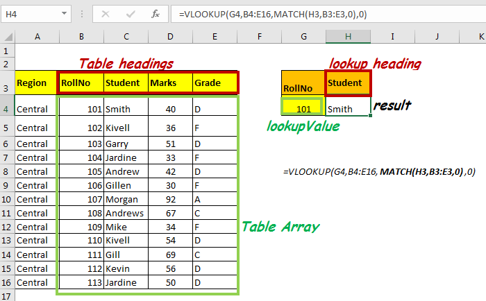
For this example, we have this table that contains data of students in range A4:E16.
Using roll no and heading, I want to retrieve data from this table. For this instance, in cell H4, I want to get data of roll no written in cell G4 and of heading in H3. If I change the heading, data from the respective range should be retrieved in cell H4.
Write this formula in cell H4
Since our table array is B4:E16, our headings array becomes B3:E3.
Note: If your data is well structured, then column headings will have the same number of columns, and it is the first row in the table.
How It Works:
So, the main part is evaluating the column index number automatically. To do so, we used the MATCH function.
MATCH(H3,B3:E3,0): Since H3 contains “student”, MATCH will return 2. If H3 had “Grade” it, it would have returned 4, and so on. The VLOOKUP formula will finally have it’s col_index_num.
As we know, the MATCH function returns the index number of a given value in the supplied one-dimensional range. Hence, MATCH will lookup for any value written in H3 in range B3:E3 and will return its index number.
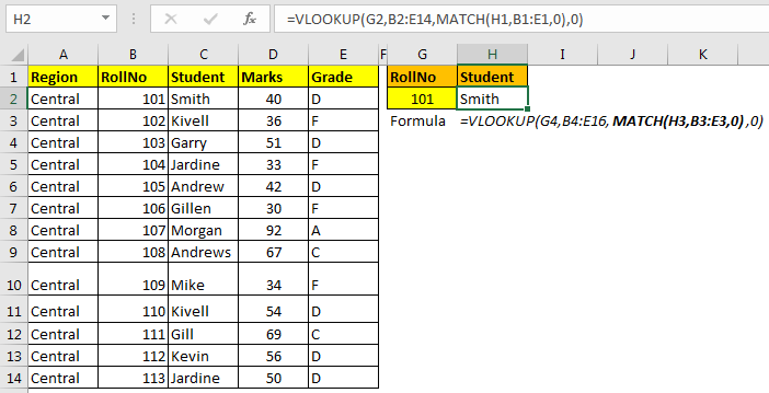
Now whenever you’ll change heading in H3, if it is in headings, this formula will return a value from the respective column. Otherwise, you’ll have an #N/A error.
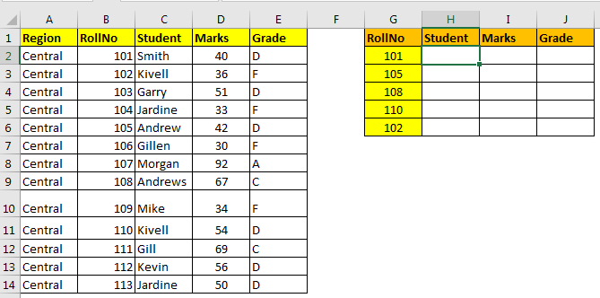
VLOOKUP in Multiple Columns Quickly
In the above example, we needed the answer from one column value. But what if you want to get multiple columns at once. If you copy the above formula, it will return errors. We need to do some minor changes in it to make it portable.
Using Absolute References with VLOOKUP
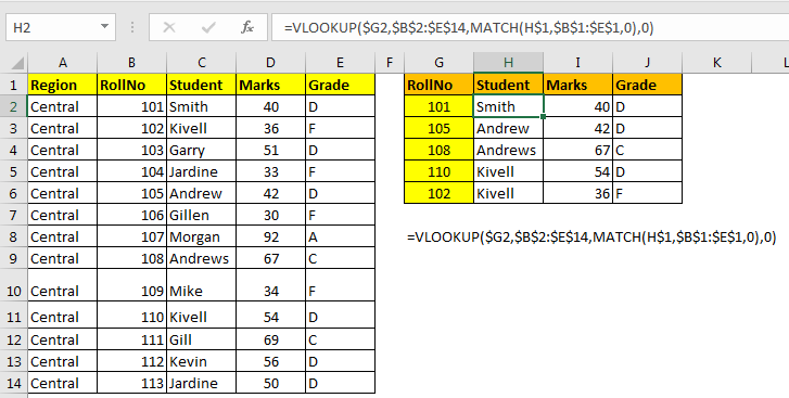
Write below formula in Cell H2.
Now copy H2 in all cells in range H2:J6 to fill it with data.
How it works:
Here I have given absolute reference of each range except row in lookup value for VLOOKUP ($G2) and column in lookup_value for MATCH (H$1).
$G2: This will allow the row to change for lookup value for VLOOKUP function while copying downwards but restrict column to change when copied to the right. Which will make VLOOKUP look for Id from G column only with the relative row.
Similarly, H$1 will allow the column to change when copied horizontally, and restrict the row when copied downwards.
Using Named Ranges
The above example works fine but gets challenging to read and write this formula. And this is not portable at all. This can be simplified using named ranges.
We will do some naming here first. For this example, I named
$B$2:$E$14 : as Data
$B$1:$E$1 : as Headings
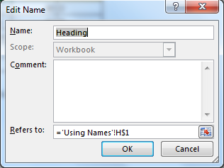
H$1 : Name it as Heading. Make the columns relative. To do so, select H1. Press CTRL+F3, click on new, in Refers to section remove '$' from the front of H.
$G2: Similarly, name it as RollNo. This time makes row relative by removing '$' from the front of 2.
Now, when you have all the names on the sheet, write this formula anywhere on excel file. It will get the correct answer always.
See, anyone can read this and understand it.
So, Using these methods, you can make col_index_num dynamic. Let me know if this was helpful in the comments section below.
Related Articles:
How to use the VLOOKUP Function in Excel
Relative and Absolute Reference in Excel
How to VLOOKUP from Different Excel Sheet
Popular Articles
50 Excel Shortcut to Increase Your Productivity : Get faster at your task. These 50 shortcuts will make you work even faster on Excel.
How to use the VLOOKUP Function in Excel : This is one of the most used and popular functions of excel that is used to lookup value from different ranges and sheets.
How to use the COUNTIF function in Excel : Count values with conditions using this amazing function. You don't need to filter your data to count specific values. Countif function is essential to prepare your dashboard.
How to use the SUMIF Function in Excel : This is another dashboard essential function. This helps you sum up values on specific conditions.
The applications/code on this site are distributed as is and without warranties or liability. In no event shall the owner of the copyrights, or the authors of the applications/code be liable for any loss of profit, any problems or any damage resulting from the use or evaluation of the applications/code.


