Introduction to VLOOKUP Function
The VLOOKUP function in Excel is without a doubt, is the most used and talked function. In any job interview that requires Excel skills, this is the most asked question that if you know how to use VLOOKUP function.
The VLOOKUP function comes under the lookup category of excel functions. The V in VLOOKUP stands for vertical. The function is used for looking up data that is structured vertically. For Horizontal lookup, there is a function called HLOOKUP.
Excel VLOOKUP function looks for the first match of a given value called lookup value, in a data table and returns the value from the given column index. The match can be approximate or exact.
Although VLOOKUP is easy to use, it has its own limitations and backdrops. We will discuss everything including the strengths and weaknesses of the function.
Syntax:
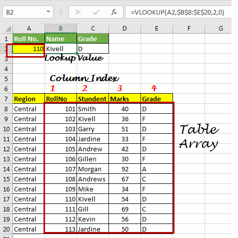
What is Lookup Value
Lookup_value: Its the value that you want to look for in a table array.
For example, if you are looking for roll no. 110 in student's table then its 110 is lookup Value.
Table_array: The table from which you want to look for lookup value.
For example, if you are looking 110 in the table array B5:E17. Then B5:E17 is your table array.
col_index_number: The column number in Table Array from which you want to fetch results.
For example if in table array B5:E17 you want get value from column D then your column index will be 3 (counting from B to D (B,C,D)).
[range_lookup]: FALSE if you want to search for exact value, TRUE if you want an approximate match.
How to Use the VLOOKUP Function
When you have a structured data and you want to lookup for data in that data, VLOOKUP function is the solution.
VLOOKUP Matching Modes
VLOOKUP has two matching modes, Approximate match and exact match. By default, VLOOKUP performs an approximate match. But if you want to force VLOOKUP function to do an exact match you can do that too. Most of the times, me and I strongly believe others too, try to do an exact match using VLOOKUP function. I don’t understand why excel developers think that users would like to use the approximate match mostly.
1. VLOOKUP Approximate Match
In VLOOKUP approximate match, if a value is not found then the last value that is less then lookup value is matched and value from given column index is returned.
VLOOKUP by default does approximate match, if we omit range lookup variable. An approximate match is useful when you want do an approximate match and when you have your table array sorted in ascending order.
Vlookup looks for the value and if it doesn’t find the value in table array then it matches the value that is less then that value in table array. Lets understand it by an Example.
Example 1
We have a student list here. Each student has scored some marks in a test. Now I want to give grade according to their marks.
Any Student who scored less than 40 should be marked F, student who scored between 40 and 60 should be marked C, and so on as shown in below image.

We would write this VLOOKUP formula in E2 and drag it down.

How It Works?
In above example our lookup values are in column D, starting from D2. The table Array is H2:I6 (note that it is sorted in ascending order and absolute). The column we are getting data from is 2. And match type we have defined approximate by passing TRUE (nothing and 1 will mean same).
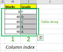
So lets examin the frist lookup value D2 that contains 40.
In this case vlookup found the exact match. Lets see next case.
The second lookup values D3 that contains 36.
This happen for each case here. For 92, last value which is less then 92 is 90. Hence A is returned for Approximate match.
2. VLOOKUP Exact Match
This most used form of VLOOKUP and may most useful too. When you want to look for exact value in first column of table array, you use exact match. For example if you are doing a lookup form a ID than you would most like want an exact match instead of any value that is less than this value.
To force VLOOKUP to a exact match in excel we pass 0 or FALSE as range_lookup parameter.
If value is not found in first column of table array the formula will return #N/A error.
Let’s see an example.
Example 2
In this example, I want to write only roll no of student in A2 and in B2 i want to fetch the student’s name and in C2 his Grade. Simple. Table array is B5:D17. Why?

So to do this, write these two formula in cell in Cell B2 and C2 respectively.
Now whichever ID you’ll write in cell A2, The VLOOKUP function will look for exact match in B column and will return value from given col_index.
How Exact Match VLOOKUP Works?
The Exact Match VLOOKUP in excel is simple. It looks for the lookup Value in first column of given table_array and returns value from value from given column_index number. If value is not found then VLOOKUP returns #N/A error.

Best Uses Of VLOOKUP Function
Vlookup has many uses. I am going to discuss some most useful use cases.
3. Use Excel VLOOKUP for Grading instead complex nested IF function
Use VLOOKUP approximate match to replace nested IF function. In Example 1 we saw how can we use vlookup to grade students according to their marks.
The VLOOKUP approximate match is faster then nested if since it uses binary search internally.
4. Use VLOOKUP to Fetch Data
This most common task that can be accomplished easily using VLOOKUP function in Excel. In example 2 we did this to fetch students data using their roll no.
5. Check if a Value is in a Record Using Vlookup.
The VLOOKUP can be used to check if a value is in some list or not.
In Example 2 when we write 152, it returns #N/A error. If VLOOKUP returns #N/A, it means that it didn’t find the given value anywhere in given data.
I have prepared a brief article on this You can read it here.
Using a VLOOKUP Formula to Check If a Value Exists
Getting Column Index Automatically
I belong to that group of people, who don’t want to repeat same task again and again. So changing col_index number again and again annoys me and I always avoid it. Actually I avoid any kind of editing in my formulas once i have written it, unless and until there is no other option.
The column index can be calculated automatically in Excel. There are several ways to do it. Let’s see some of’em here.
6. Use VLOOKUP Function With MATCH Function
So as we know that MATCH function return the found index of matched value.
So if we have exactly same headings at lookup location as the source data, than we can use to get col_index. How? Let us see..
In below data, we want to just write roll number in G2 and want to fetch Student name, marks and grade in H2, whichever heading we write there.
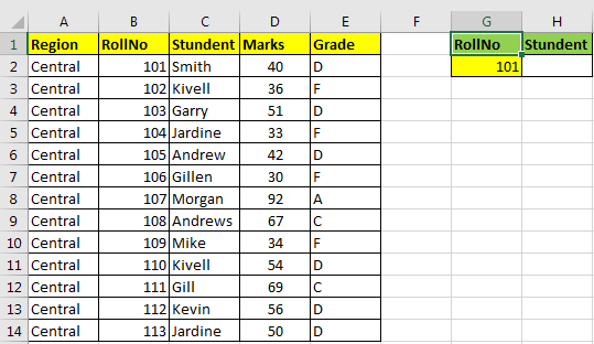
Write this formula in cell H2
Now whenever you will change Heading in H1 that value in H2 will be shown from that column.
You can use a drop down using data validation that has all heading from table, to make it more user friendly.

Here VLOOKUP is doing exact match. Now VLOOKUP is doing its usual stuff of pulling data. The magic is done by MATCH function at col_index position.
Here VLOOKUP sees for any value in G2 in first column of table array B2:E14. Now at the place of col_index we have MATCH(H1,B1:E1,0).
MATCH function looks for any value in H1 in range B1:E1 and returns index of match value.
For example when we type student in H1 it look for it in range B1:E1. It is found in C2. hence it returns 2. If we type Grade it will return grade of student.
Note that when we type Region, it return #N/A. Because it is out of scope of the table. We will talk about it latter in the article.
This is the best way to make VLOOKUP automatic. There are other methods to but they are not that flexible than this.
7. Use VLOOKUP Function With COLUMN Function
The column function returns the column number of supplied reference. And what we need for fetching data using VLOOKUP? Col_index. So using COLUMN function we can of course get data from any data set.
Let’s take the above example. But now we need to retrieve whole data. Not just one column.
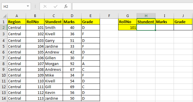
Write this Formula in H2 and copy in I2 and J2.
This will give you a dynamic result. How? Lets see.
The VLOOKUP works as usual. At column_index we have written COLUMN(B1), which will translate to 2, since we have student name in 2 column from B column, it returns name of student.
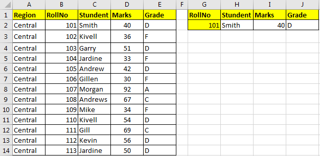
Important: This works because we have our table starting from B column. If your table in middle of sheet, then you’ll need to subtract or add some numbers so that it matches your requirement.
For example, if the above table were starting from C1 in same structure then all below formulas were work fine.
8. VLOOKUP to Merge Data
In most databases there is one query that merges to tables, mostly called a join query but MS Excel in no database hence it doesn’t have join query. But this doesn’t mean we can not join two table if we have some common columns in two tables.
So when you get some data from two departments of same company, you would want to merge them in order to analyse that data.
For example, when you get marks of students from teachers and then attendance record from administrative department, you would want to see which student got what grade and what is his attendance percentage, in once place.

We need to merge them in below table.

Marks, we need to get from Marks Table, and Attendance from Attendance Data.
Write below Formulas in Cell D19 to get Marks and drag down.
Write Below Formula in Cell E19

And we have merged two tables into one table. You can add more than two tables of course. You just need to get data from all the tables you want at one place using VLOOKUP.
Best Practices of VLOOKUP
So, all above examples we just used vlookup with raw data. In all above examples, we were careful about the data we were using. We needed to be careful, while giving references of table arrays. But there are certain ways, that can reduce this effort extensively.
9. Use Absolute References with VLOOKUP
You may have noticed, that in some articles I have used absolute ranges (range $ sign). Well, absolute rages are used when we don’t want range to be changed while copying formula cell to other cells.
For example, if I have =VLOOKUP(G2,B2:E14,2,0),0) in cell H2, and if I copy or drag down it in cell H3 the formula will change to =VLOOKUP(G3,B3:E15,2,0). All references are changed relatively. Here we may want to change reference of lookup value but not the table array. Because B2 gets out or range and we may want have it in our table arrays always.
So, to prevent that we use absolute references. We make those ranges absolute that we don’t want to change, like table_array in H2, =VLOOKUP(G2,$B$2:$E$14,2,0),0). When you copy H2 in H3 the formula will be =VLOOKUP(G3,$B$2:$E$14,2,0),0). Note that lookup value is changed but not table_array.

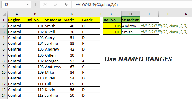
In above example, we used absolute referencing for fixing the table_array. It is quite looks fuzzy and hard to read. How about if you can just write ‘data’ at place of $B$2:$E$14 and it would reference at $B$2:$E$14 always. It will make it even easier to read and write the formula.
So just select the range and name it ‘data’.
To name a range, select the range. Right click, click on Define Name and name the range you want. Now just =VLOOKUP(G3,data,2,0),0) formula will work exactly same as previously.
You can read more about named ranges in Excel. I have explained each and every aspect of named range here.
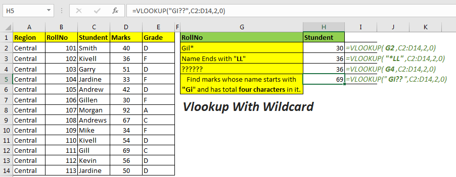
VLOOKUP allows partial matching. Yes, while doing exact match of VLOOKUP you can use wildcard operators to do partial matching. For example, if you want to lookup a value that starts with ‘Gil’, you can use wildcard operator * with ‘Gil’ as “Gil*”. Let’s see an example.
Here I want to get marks of student whose name starts with Gil. To get so, I will write below formula.
There are two wildcards are available in excel to use with VLOOKUP function.
Asterisk (*) wildcard. This is used when, user is does not know number of characters there are and only know some characters of match. For example if user knows a name that starts with “Sm”, then he will write “Sm*”. If user know that a lookup value that ends with “123” then he will write “*123”. (wild card only works with texts). And of he know that “se” comes inside a text then he will write “*se*”.

Question Mark (“?”). This is used when the user knows the number of characters missing. For example, if I want to look up a value that has 4 characters in it but I don’t know what they are I will simply write “????” at the place of the lookup value.
Vlookup will returns respective value of first found value that has exactly four characters in it.
Important: Wild card works only with text values. Convert numbers to text if you want to use wildcard with them.
VLOOKUP indeed is a powerful and easy function for fetching values but there are many areas where VLOOKUP is just not that helpful. If you are working on excel, you must know them too and how to do task that VLOOKUP can’t do.
12. Can’t Fetch Value From Left of Table_Array
The biggest flaw of VLOOKUP function is that, it can’t fetch value from left of table array. VLOOKUP only lookups right of the lookup value.
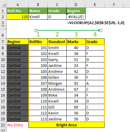
This is because, VLOOKUP searches for given lookup value in first column of given table array. It will never return a value from outside of the table. And if try to keep left column in table array, it becomes the first column of table array, hence lookup value will be searched in that range. Which will probably generate error.
To lookup values from left of a lookup value we use INDEX-MATCH instead. The INDEX-MATCH function can lookup values from any column on sheet. Actually, lookup range and the range from which you want to lookup values are totally independent, which makes index match highly customizable.
VLOOKUP returns #N/A even when lookup value exist.
#N/A error is returned by VLOOKUP function when the lookup value is not found. You may find it annoying when a value exists in range but VLOOKUP returns #N/A error.
14. When Numbers are Formated as Text
This mostly happens when numbers are formated as text. When you find using CTRL+F command excel will find it, but when you try to use VLOOKUP, it returns #N/A. This task is given in most interviews as trick questions.
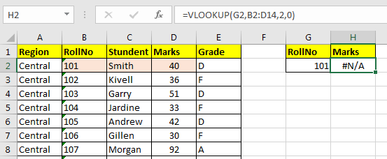
In the above image, you can see that 101 is right there, but the formula is returning an error. How, do you handle it? Well, there are two methods.
1.Convert text to number in data
You can see that green tag in left upper corner in rollno column. They indicate that something is unusual in the value of cell. When you select the cell, it will show that number is formated as text.
When you click on the exclamation mark (!), it will show you option of Convert To Number. Select all cells and click on this option. All values will be converted to text.
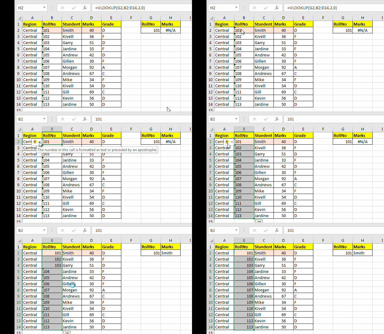
2. Convert your lookup number into text in formula
In the above example, we mutated original data. You may not want to change anything in original data. So you would want do this in formula instead. To do change number into text in VLOOKUP formula write this.
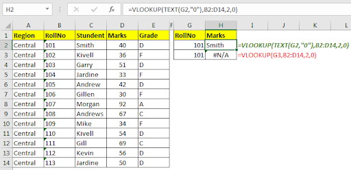
Here formula dynamically changes number into text and then matches it with given range.
15. Text Having Leading and Trailing Spaces
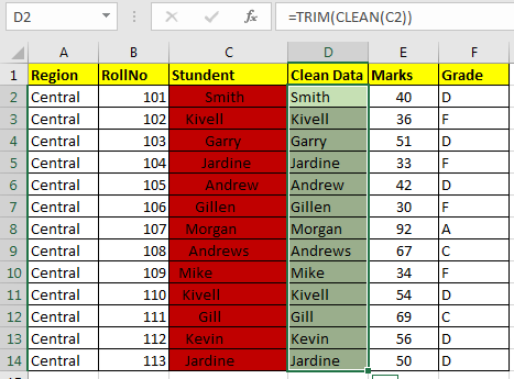
Some data provided by data entry operators and data from internet are not clean. They may have trailing spaces or some unprintable characters. While doing lookup using these values, you may see some #N/A error. To avoid this, clean your data first. To remove leading spaces use TRIM function. TRIM removes any number of leading or trailing spaces from text.
So, i suggest you add a new column and get your cleaned data there. Then value paste it. Now if you want, you can get rid of the original column.
Handling Errors of VLOOKUP
As you know, VLOOKUP fails to find a value, it returns a #N/A error. Well it’s ok to get #N/A error, maybe you sometimes intend to get so, like when you want to check if the a value already exists in list or not. There #N/A signifies that the value is not there.
But #N/A looks ugly. How about getting a user friendly output, like “Id not found” or “Customer not Found”. We can use IFERROR with VLOOKUP function to avoid #N/A.
Use below formula to trap error in VLOOKUP.
16. VLOOKUP with MULTIPLE Criterias
VLOOKUP can’t work with multiple criterias. Yes, you can only have one criterion to lookup values using the VLOOKUP formula.
For example, if you have the first name and last name in two separate columns.
And now if you want to lookup value whose first name is John and Last name Dave, then you can’t do it normally.
But there’s a workaround for this. You can create a separate column by concatenating first name and last name and then look up at that first and last name column.
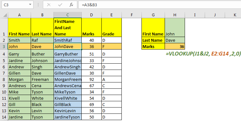
There is an INDEX-MATCH alternative that can lookup multiple criteria without any helping column.
17. VLOOKUP Retrieves First Found Value only
Imagine you have some data in the central region. Now you want to get the first 5 data records of the central region. The VLOOKUP will only return the first central value in all five records. This is a major backdrop.

But it doesn’t mean we can’t achieve this. We can use a complex arrays formula as below.
Write this formula and hit CTRL+SHIFT+ENTER.
And its done.
I have explained it in article how to LOOKUP multiple values in Excel.
So yeah guys, in this article I have covered all possible aspects of VLOOKUP function as per my knowledge. If you think I have missed something than please let me know in the comments section below.
Related You May Like:
Vlookup Top 5 Values with Duplicate Values Using INDEX-MATCH in Excel
VLOOKUP with Dynamic Col Index
Partial match with VLOOKUP function
Use VLOOKUP from Two or More Lookup Tables
Using a VLOOKUP Formula to Check If a Value Exists
How to VLOOKUP from Different Excel Sheet
The applications/code on this site are distributed as is and without warranties or liability. In no event shall the owner of the copyrights, or the authors of the applications/code be liable for any loss of profit, any problems or any damage resulting from the use or evaluation of the applications/code.
What's up, every time i used to check webpage posts here in the early hours in the daylight, since i
love to find out more and more.