It's easy to look up for value with one unique key in a table. We can simply use the VLOOKUP function. But when you don’t have that unique column in your data and need to lookup in multiple columns to match a value, VLOOKUP doesn’t help.
So, to lookup a value in a table with multiple criteria we will use INDEX-MATCH-INDEX formula.

Generic Formula for Multiple Criteria Lookup
lookup_range: Its the range from which you want to retrieve value.
Criteria1, Criteria2, Criteria N: These are the criteria you want to match in range1, range2 and Range N. You can have up to 270 criteria - range pairs.
Range1, range2, rangeN : These are the ranges in which you will match your respective criteria.
How it will work? Let's see…
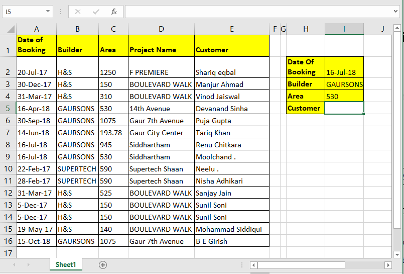
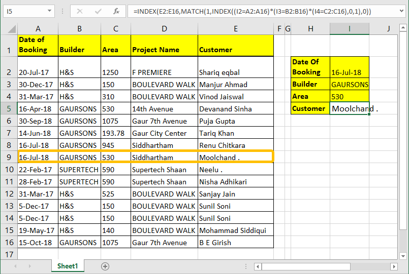
Here I have a data table. I want to pull the name of the customer using Date of Booking, Builder and Area. So here I have three criteria and one lookup range.

Write this formula in cell I4 hit enter.

How it works:
We already know how INDEX and MATCH function work in EXCEL, so i am not going to explain that here. We will talk about the trick we used here.
(I1=A2:A16)*(I2=B2:B16)*(I3=C2:C16): The main part is this. Each part of this statement return an array of true false.
When boolean values are multiplied they return array of 0 and 1. Multiplication works as AND operator. Hense when all value are true only then it returns 1 else 0
(I1=A2:A16)*(I2=B2:B16)*(I3=C2:C16) This altogether will return
{FALSE;FALSE;FALSE;FALSE;FALSE;FALSE;TRUE;TRUE;FALSE;FALSE;FALSE;FALSE;FALSE;FALSE;FALSE}*
{FALSE;FALSE;FALSE;TRUE;TRUE;TRUE;TRUE;TRUE;FALSE;FALSE;FALSE;FALSE;FALSE;FALSE;TRUE}*
{FALSE;FALSE;FALSE;TRUE;FALSE;FALSE;FALSE;TRUE;FALSE;FALSE;FALSE;FALSE;FALSE;FALSE;FALSE}
Which will translate into
{0;0;0;0;0;0;0;1;0;0;0;0;0;0;0}
INDEX((I1=A2:A16)*(I2=B2:B16)*(I3=C2:C16),0,1): INDEX Function will return the same array ({0;0;0;0;0;0;0;1;0;0;0;0;0;0;0}) to MATCH function as lookup array.
MATCH(1,INDEX((I1=A2:A16)*(I2=B2:B16)*(I3=C2:C16),0,1): MATCH function will look for 1 in array {0;0;0;0;0;0;0;1;0;0;0;0;0;0;0}. And will return index number of first 1 found in array. Which is 8 here.
INDEX(E2:E16,MATCH(1,INDEX((I1=A2:A16)*(I2=B2:B16)*(I3=C2:C16),0,1),0)): Finally, INDEX will return value from given range (E2:E16) at found index (8).
Simple????. Sorry, couldn’t make it more simpler.
If you can hit CTRL + SHIFT + ENTER consequently then you can eliminate the inner INDEX function. Just write this formula and hit CTRL + SHIFT + ENTER.
Generic Array Formula for Multiple Criteria Lookup
Formula works same as above explanation.
I tried my best to explain it as simple as possible. But if I was not clear enough, let me know it in the comment section below. By the way, you don’t need to know how the engine works to drive a car. You just need to know how to drive it. And you know it very well.
Related Articles:
How to Lookup Top 5 Values with Duplicate Values Using INDEX-MATCH in Excel
How to VLOOKUP Multiple Values in Excel
How to VLOOKUP with Dynamic Col Index in Excel
How to use VLOOKUP from Two or More Lookup Tables in Excel
Popular Articles:
50 Excel Shortcuts to Increase Your Productivity
How to use the VLOOKUP Function in Excel
The applications/code on this site are distributed as is and without warranties or liability. In no event shall the owner of the copyrights, or the authors of the applications/code be liable for any loss of profit, any problems or any damage resulting from the use or evaluation of the applications/code.
This seems simpler:
= IF( (Criteria1) * (Criteria2) * (Criteria3), ReturnColumn)
I believe my multiplication formula above, doesn't work. I don't know what i was thinking either.
I was just doing this - searching a large excel spreadsheet for a list of values and (of course) after I finished that 2 hours of work, thought of this;
If you set the entire sheet to "highlight duplicate values", then paste the list into the spreadsheet - it will highlight any that are already in there. Not professional, but, it works 🙂