
In this article, we will learn how to Lookup & SUM values with INDEX and MATCH function in Excel.
For the formula to understand first we need to revise a little about the three functions
SUM function adds all the numbers in a range of cells and returns the sum of these values.
INDEX function returns the value at a given index in an array.
MATCH function returns the index of the first appearance of the value in an array ( single dimension array ).
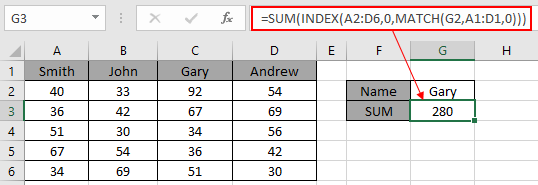
Now we will make a formula using the above functions. Match function will return the index of the lookup value in the header field. The index number will now be fed to the INDEX function to get the values under the lookup value.
Then the SUM function will return the sum from the found values.
Use the Formula:
The above statements can be complicated to understand. So let’s understand this by using the formula in an example
Here we have a list of marks of students and we need to find the total marks for a specific person (Gary) as shown in the snapshot below.
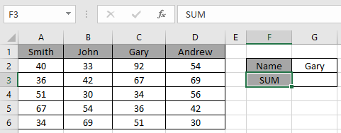
Use the formula in the C2 cell:
Explanation:
Here values to the function is given as cell reference.
As you can see in the above snapshot, we got the SUM of the marks of student Gary. And it proves the formula works fine and for doubts see the below notes for understanding.
Notes:
Hope you understood how to use the LOOKUP function in Excel. Explore more articles on Excel lookup value here. Please feel free to state your queries below in the comment box. We will certainly help you.
Related Articles
Use INDEX and MATCH to Lookup Value
How to use the SUM function in Excel
How to use the INDEX function in Excel
How to use the MATCH function in Excel
How to use LOOKUP function in Excel
How to use the VLOOKUP function in Excel
How to use the HLOOKUP function in Excel
Popular Articles
The applications/code on this site are distributed as is and without warranties or liability. In no event shall the owner of the copyrights, or the authors of the applications/code be liable for any loss of profit, any problems or any damage resulting from the use or evaluation of the applications/code.


