
The excel’s VLOOKUP function isn’t case sensitive and it will return the fist matched value from the list. INDEX-MATCH is no exception but it can be modified to make it case sensitive. Let’s see how.
Generic Formula for Case Sensitive Lookup
It’s an array formula and need to be entered with CTRL+SHIFT+ENTER.
Result_array : The index from which you want to get results.
Lookup_value: the value which you are looking for in lookup_array.
Lookup_array: The array in which you will look for lookup value:
Let’s learn by an example.
Example: Do an EXACT INDEX MATCH to lookup case sensitive value
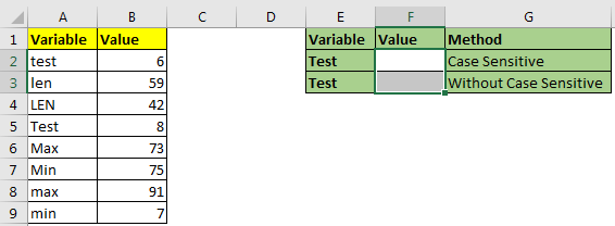
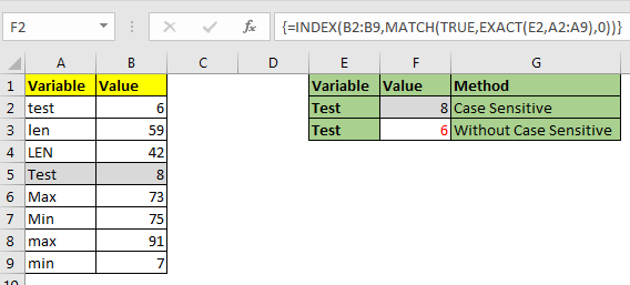
Here we have this data of variables. These variables are case sensitive. I Mean “test” and “Test” are two different values. We need to retrieve “Test”’s value from the list. Let’s implement above generic formula on this example.
Write this formula in cell F2. This formula is an array formula and need to be entered with CTRL+SHIFT+ENTER.
This returns the value 8 which is at 5th position. If we had used VLOOKUP or simple INDEX-MATCH, it would have returned 6 which is first test in list.

How does it work?
It’s a simple INDEX-MATCH. The trick is use of the EXACT function in this formula.
EXACT(E2,A2:A9): The EXACT function is used form matching case sensitive letters. This part looks for E2’s Value (“Test”) in range A2:A9 and returns an array of TRUE and FALSE. {FALSE;FALSE;FALSE;TRUE;FALSE;FALSE;FALSE;FALSE}.
Next in MATCH(TRUE,{FALSE;FALSE;FALSE;TRUE;FALSE;FALSE;FALSE;FALSE},0) part, Match looks for TRUE in array returned above. It finds the first true at 4th position and returns 4.
Finally the formula is simplified to INDEX(B2:B9,4). It looks at 4th row in B2:B9 and returns the value it contains. Which is 8 here.
So yeah guys, this how you do case sensitive lookup in excel. Let me know if you have any doubts regarding this topic or any other excel topic. The comments section is all yours.
Related Articles:
Use INDEX and MATCH to Lookup Value
How to Use LOOKUP function in Excel
Lookup Value with Multiple Criteria
Popular Articles:
The applications/code on this site are distributed as is and without warranties or liability. In no event shall the owner of the copyrights, or the authors of the applications/code be liable for any loss of profit, any problems or any damage resulting from the use or evaluation of the applications/code.


