
In this article, we will learn How to Filter by selected cells in Excel.
Scenario:
In Excel, Apply Filtering is a simple, however, amazing & powerful way to analyze data. Advanced filters are quite easy to use. Here's how you can use Excel's advanced filtering capabilities.
In this article we have created tutorials of advanced filters, in which you can learn how to use formulas and functions for filters and how to use advanced filters. Below you can find different ways of filter.
Filter by in Excel
filter the data as per the selected cell on Excel workbook. Find different filtering options as mentioned below.
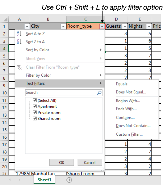
Select any table header cell and Access Filter using Home > Sort & Filter > Filter or just use Ctrl + Shift + Enter from keyboard.
You can filter by:
Example :
All of these might be confusing to understand. Let's understand how to use the function using an example. Here we have a table and we need to see what all types filter an excel user can access.
First of all select any table header and Use Ctrl + Shift + Enter to apply filters. This will enable a drop down option on all column headers.
One of the important features is to filter values by background cell color. This excel option stores all the different color values. Just click the arrow key, this will open the filter table for the selected cell.
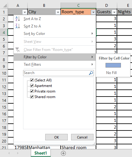
As you can see here we can filter all blue colored records just by two clicks. Now we learn how to filter by text or numbers value.
Filter by text or number
Excel records text and numbers data separately. In a text column, excel allows only text filters as shown below
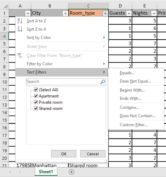
Here as you can see there are only text filter values that are allowed to filter. But notice as we switch to the Numbers column it changes to numbers filters as shown below.
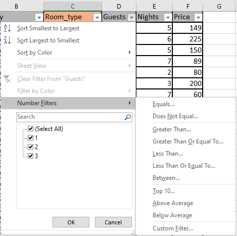
As you can see the number filter now clearly. You can also access sort values using Colour in Excel.
Here are all the observational notes using the formula in Excel
Notes :
Hope this article about How to Filter by selected cell in Excel is explanatory. Find more articles on calculating values and related Excel formulas here. If you liked our blogs, share it with your friends on Facebook. And also you can follow us on Twitter and Facebook. We would love to hear from you, do let us know how we can improve, complement or innovate our work and make it better for you. Write to us at info@exceltip.com.
Related Articles :
How to Filter the Data in Excel using VBA : Filtering data using VBA is easy. These simple lines of codes filter the data on the given criteria.
How to use the SUBTOTAL function in Excel : Returns the SUM, COUNT, AVERAGE, STDEV or PRODUCT on applied filtered data in Excel.
How to use the Filter Function in Excel 365 (new version) : The FILTER function returns the filtered table by the given column number and condition. The function also works with data in a horizontal manner.
How to use the SORT Function in Excel 365 (new version) : The SORT function returns the sorted array by the given column number in the array. It also works on horizontal data.
Sort Numeric Values with Excel RANK Function : To sort the numeric values we can use the Rank function. The formula is
Excel Formula to Sort Text : To sort text values using formula in excel we simply use the COUNTIF function. Here is the formula.
How to Delete only Filtered Rows without the Hidden Rows in Excel : Many of you are asking how to delete the selected rows without disturbing the other rows. We will use the Find & Select option in Excel.
Popular Articles :
50 Excel Shortcuts to Increase Your Productivity : Get faster at your tasks in Excel. These shortcuts will help you increase your work efficiency in Excel.
How to use the VLOOKUP Function in Excel : This is one of the most used and popular functions of excel that is used to lookup value from different ranges and sheets.
How to use the IF Function in Excel : The IF statement in Excel checks the condition and returns a specific value if the condition is TRUE or returns another specific value if FALSE.
How to use the SUMIF Function in Excel : This is another dashboard essential function. This helps you sum up values on specific conditions.
How to use the COUNTIF Function in Excel : Count values with conditions using this amazing function. You don't need to filter your data to count specific values. Countif function is essential to prepare your dashboard.
The applications/code on this site are distributed as is and without warranties or liability. In no event shall the owner of the copyrights, or the authors of the applications/code be liable for any loss of profit, any problems or any damage resulting from the use or evaluation of the applications/code.


