
In this article, we will learn How to consolidate lists in Excel.
Why Consolidate?
Whenever we have the same type of data over different sheets. Like Add all the Daily amounts of milk, coffee and tea to get the total of all amounts having milk, coffee and tea. Consolidate means to join things together into one. So consolidate the whole data using Consolidate in excel.
Consolidate in Excel
Select the new sheet where you need the consolidated data be. Then Go to Data > Consolidate.
Choose the aggregate function > select and add all data reference > Tick Top row & Left label > Click Ok.
Example :
All of these might be confusing to understand. Let's understand how to use the function using an example. Here we have products data from different categories having sales, quantity and Profit. We need to sum all sales, quantity and profit for all three sheets.
Sheet1 :

Sheet2 :

Sheet3 :

These tables are named as data1, data2 and data3 as seen clearly from the top left Name box. Use this for efficient use of consolidating tables
Now we use the consolidate option. Insert a new sheet And Go to Data > Consolidate.

Consolidate dialog box appears.

Choose the Function from the list. List has Sum, Count, Average, Max, Min, Stdev, Var to calculate the fields. Here we choose SUM function.

In the Reference box, select the table and click Add to merge it. If using named ranges, just type data1 > Add > type data2 > Add > type data3 > Add.
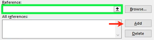
Similarly add all data in sheet1, sheet2, sheet3 one by one. Tick the top row box, tick the left column box and tick Create link to source data box.

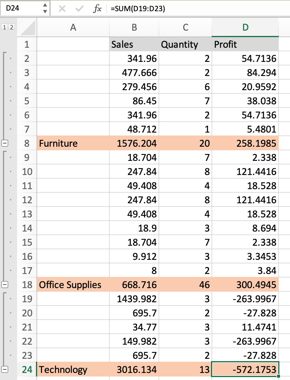
Now click Ok to get the whole sum sales, quantity and Profit based on Category column.

This is Level of grouped data. Switch to Level 2 for detailed sum.
![]()
As you can see clearly the SUM of values with different categories. Isn't it easy. Selecting all data by reference may be hectic. So just name the table as data1, data2 and data3 as used in the explained example.
You can also use the SUMIF function. It works with one criteria and SUM values based on the criteria. But Consolidate option allows user to choose from various aggregate function
Here are all the observational notes using the formula in Excel
Notes :
Hope this article about How to use the ... function in Excel is explanatory. Find more articles on calculating values and related Excel formulas here. If you liked our blogs, share it with your friends on Facebook. And also you can follow us on Twitter and Facebook. We would love to hear from you, do let us know how we can improve, complement or innovate our work and make it better for you. Write to us at info@exceltip.com.
Related Articles :
Relative and Absolute Reference in Excel : Understanding of Relative and Absolute Reference in Excel is very important to work effectively on Excel. Relative and Absolute referencing of cells and ranges.
All About Excel Named Ranges : excel ranges that are tagged with names are easy to use in excel formulas. Learn all about it here.
How to use Shortcut Keys for Sort & filter in Excel : Use Ctrl + Shift + L from keyboard to apply sort and filter on table in Excel.
Excel VBA Variable Scope : In all the programming languages, we have variable access specifiers that define from where a defined variable can be accessed. Excel VBA is no Exception. VBA too has scope specifiers.
How to Dynamically Update Pivot Table Data Source Range in Excel : To dynamically change the source data range of pivot tables, we use pivot caches. These few lines can dynamically update any pivot table by changing the source data range. In VBA use pivot tables objects as shown below.
50 Excel Shortcuts to Increase Your Productivity : Get faster at your tasks in Excel. These shortcuts will help you increase your work efficiency in Excel.
Popular Articles :
How to use the IF Function in Excel : The IF statement in Excel checks the condition and returns a specific value if the condition is TRUE or returns another specific value if FALSE.
How to use the VLOOKUP Function in Excel : This is one of the most used and popular functions of excel that is used to lookup value from different ranges and sheets.
How to use the SUMIF Function in Excel : This is another dashboard essential function. This helps you sum up values on specific conditions.
How to use the COUNTIF Function in Excel : Count values with conditions using this amazing function. You don't need to filter your data to count specific values. Countif function is essential to prepare your dashboard.
The applications/code on this site are distributed as is and without warranties or liability. In no event shall the owner of the copyrights, or the authors of the applications/code be liable for any loss of profit, any problems or any damage resulting from the use or evaluation of the applications/code.


"Who is in the top, in the bottom?
why I must sort it ?"