How to Draw Lines between Sorted Groups in Excel

In this article, we will learn How to Draw Lines between Sorted Groups in Excel.

Why do we use conditional formatting to highlight cells in Excel ?

Conditional Formatting is used to highlight the data on the basis of some criteria. It would be difficult to see various trends just for examining your Excel worksheet. Conditional Formatting provides a way to visualize data and make worksheets easier to understand. It allows you to apply the formatting basis on the cell values such as colours, icons and data bars.

Excel Conditional formatting gives you inbuilt formulation like Highlight cells rules or top/bottom rules. These will help you achieve formulation using simple steps.

Choose the New rule to create a customized formula for highlighting cells. For example Highlight sales values where sales values are in between 150 to 1000. For this we use Conditional formatting. Try the formula in adjacent cells before applying in the conditional formatting formula box.

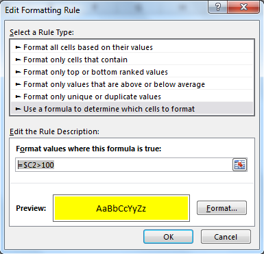
Formula box in Conditional formatting

After selecting the New rule in conditional formatting. Select the Use a formula to determine which cells to format -> it will open the formula box as shown in the image above. Use the formula in it and select the type of formatting to choose using Format option (like Yellow background as shown in the image). 

To draw lines between sorted groups of data:

1. Sort the List by Customer Name by selecting a cell in column C (see screenshot)

and clicking Sort Smallest to Largest icon (in Data tab).

2. Select a cell in the List and press Ctrl+Shift+* or press Ctrl+A.
3. Select Home -> Conditional Formatting (in Styles Group) -> New Rule.
4. Select Use a Formula to determine which cells to format.
5. In Format values where this formula is true enter the formula =$C1>$C2,

click the Format button, select the Border tab, in Border section choose a color

and click Underline, then click OK twice.

Example :

All of these might be confusing to understand. Let's understand it better via running the formula on some values. Here we have some university exam codes. We need to highlight the mathematics exam codes. Mathematics Exam code begins with "MA".

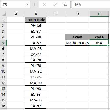
What we need here is to check each cell which starts with "MA".

Go to Home -> Conditional formatting -> New Rule

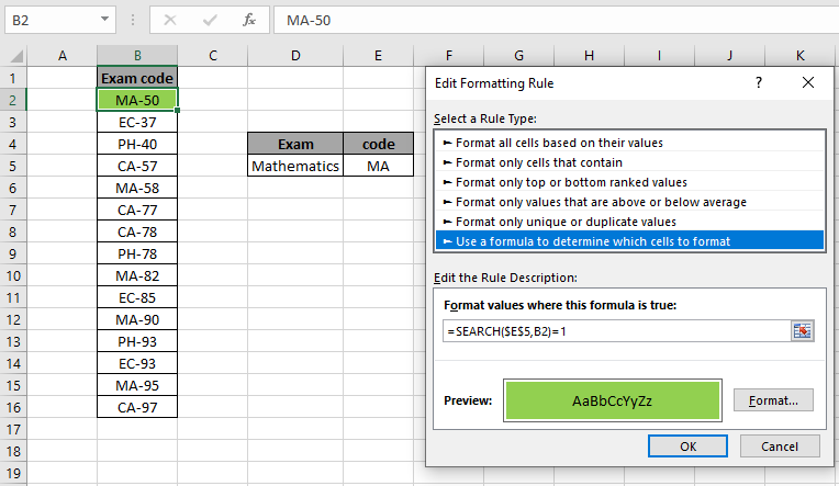
A dialog box appears in front select Use a formula to determine which cells to format -> input the below formula under the Format values where this formula is True:

Use the formula:

Explanation:

1. Search matches the string in the cell value.
2. Search function returns the position of occurrence of the substring in text.
3. If the position matches with 1 i.e. the start of the cell. The formula returns True if matched or else False.
4. True value in conditional formatting formats the cell as required.
5. Customize the cell format by clicking the Format button in the right bottom of the dialog box as shown below.
6. The format will will displayed adjacent to the Format button.

The background color gets Green ( highlight formatting) as you click Ok as shown above. Now copy the formula to the rest of cells using the Ctrl + D or dragging down form right bottom of B2 cell.

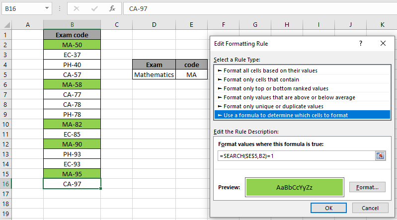
As you can see all the mathematics exam codes are highlighted. You can input specific value substring, with quotes(") in the formula along with an example solved using the FIND function.

Here are all the observational notes regarding using the formula.

Notes:

1. Conditional formatting allows you to apply the formatting basis on the cell values such as colours, icons and data bars.
2. The formula works for text and numbers both.
3. SEARCH function is case insensitive function.

Hope this article about How to Draw Lines between Sorted Groups in Excel is explanatory. Find more articles on highlighting cells and related Excel formulas here. If you liked our blogs, share it with your friends on Facebook. And also you can follow us on Twitter and Facebook. We would love to hear from you, do let us know how we can improve, complement or innovate our work and make it better for you. Write to us at info@exceltip.com.

Related Articles:

Find the partial match number from data in Excel : find the substring matching cell values using the formula in Excel

How to Highlight cells that contain specific text in Excel : Highlight cells based on the formula to find the specific text value within the cell in Excel.

Conditional formatting based on another cell value in Excel : format cells in Excel based on the condition of another cell using some criteria.

IF function and Conditional formatting in Excel : How to use IF condition in conditional formatting with formula in excel.

Perform Conditional Formatting with formula 2016 : Learn all default features of Conditional formatting in Excel

Conditional Formatting using VBA in Microsoft Excel : Highlight cells in the VBA based on the code in Excel.

Popular Articles :

How to use the IF Function in Excel : The IF statement in Excel checks the condition and returns a specific value if the condition is TRUE or returns another specific value if FALSE.

How to use the VLOOKUP Function in Excel : This is one of the most used and popular functions of excel that is used to lookup value from different ranges and sheets.

How to use the SUMIF Function in Excel : This is another dashboard essential function. This helps you sum up values on specific conditions.

How to use the COUNTIF Function in Excel : Count values with conditions using this amazing function. You don't need to filter your data to count specific values. Countif function is essential to prepare your dashboard.