
With VLOOKUP we always get the first match. The same happens with the INDEX MATCH function. So how do we VLOOKUP second match or 3rd or nth? In this article, we will learn, how to get the Nth occurrence of a value in range.
Generic Formula
Note: this is an array formula. You need to enter it with CTRL + SHIFT + ENTER.
Range: the range in which you want to lookup nth position of value.
Value: the value of which you are looking nth position in the range.
First_cell_in_range: the first cell in the range. If the range is A2:A10 then the first cell in the range is A2.
n: the occurrence number of values.
Let’s see an example to make things clear.
Example: Find the Second Match in Excel
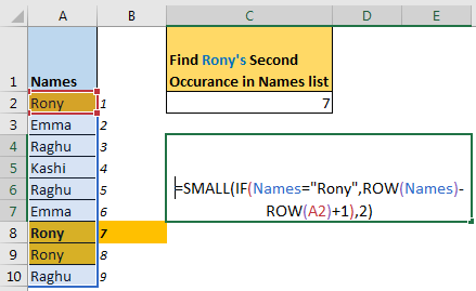
So here I have this list of names in excel range A2:A10. I have named this range as names. Now I want to get the position of the second occurrence of “Rony” in names.

In the image above, we can see it is on 7th position in range A2:A10 (names). Now we need to get its position using an excel formula.
Apply the above generic formula in C2 to lookup the second occurrence of Rony in the list.
Enter it with CTRL + SHIFT + ENTER..

And we have an answer. It is showing 7, which is correct. If you change the value of n to 3 it will give 8. If you change the value of n greater than the occurrence of the value in the range, it will return #NUM error.
How does it work?
Well, it is quite easy. Let’s see each part one by one.
IF(names=“Rony” ,ROW(names)-ROW(A2)+1) :
In IF, names=“Rony” returns an array of TRUE and FALSE. TRUE whenever a cell in range names (A2:A10) matches to “Rony”.{TRUE;FALSE;FALSE;FALSE;FALSE;FALSE;TRUE;TRUE;FALSE}.
ROW(names): here ROW function returns the row number of each cell in names. {2;3;4;5;6;7;8;9;10}.
ROW(names)-ROW(A2)Then we subtract row number of A2 from each value in the given array. This gives us an array of serial numbers starting from 0. {0;1;2;3;4;5;6;7;8}.
ROW(names)-ROW(A2)+1: To get serial numbers starting from 1, we add 1 to each value in this array. This gives us the serial number starting from 1. {1;2;3;4;5;6;7;8;9}.
Now we have IF({TRUE;FALSE;FALSE;FALSE;FALSE;FALSE;TRUE;TRUE;FALSE},{1;2;3;4;5;6;7;8;9}). This solves to {1;FALSE;FALSE;FALSE;FALSE;FALSE;7;8;FALSE}.
Now we have formula solved to SMALL({1;FALSE;FALSE;FALSE;FALSE;FALSE;7;8;FALSE},2). Now SMALL returns the second smallest value in the range, which is 7.
How do we use it?
The question arrives: what is the benefit of getting a raw index of the nth match? It would be more useful if you could retrieve related information from nth value. Well, that can be done too. If we want to get value from the adjacent cell’s value of nth match in range names (A2: A10).
So yeah guys, this is how you can get the nth match in a range. I hope I was explanatory enough. If you have any doubts regarding this article or any other excel/VBA related topic, write in the comments section below.
Related Articles:
How To Get Sequential Row Number in Excel
Vlookup Top 5 Values with Duplicate Values Using INDEX-MATCH in Excel
Use INDEX and MATCH to Lookup Value
Lookup Value with Multiple Criteria
Popular Articles:
The applications/code on this site are distributed as is and without warranties or liability. In no event shall the owner of the copyrights, or the authors of the applications/code be liable for any loss of profit, any problems or any damage resulting from the use or evaluation of the applications/code.


