
Categorising string based on some words was one of my basic task in data analysis. For example, in a survey if you ask people what they like about a particular smart phone, the same answers will have a variety of words. For camera, they may use the words like photos, videos, selfies etc. They all imply camera. So it is very important to categorize sentences before, to get some meaningful information.

In this article, we will learn how to categorize in excel using keywords.
Let’s take the example of survey we talked about.
Example: Categorize Data Gathered From a Survey in Excel
So, we have done a survey about our new smartphone xyz. We have asked our customers what they like about xyz phone and captured their response in excel. Now we need to know who liked our LED screen, speaker and camera.

For this, we have prepared a list of keywords that may refer to a category, as you can see in below image. To understand, I have kept it small.
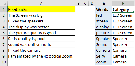
The Feedbacks is in range A2:A9, keywords are in E2:E10 and Category is in F2:F10.
The generic formula to create categories will be:
Note the curly braces, it is a array formula. Needs to be entered using CTRL+SHIFT+ENTER.
Category: It is the range that contains list of categories. Sentences or feedbacks will be categorised by these values. In our case it is F2:F10.
Words: it is the range that contains list of keywords or phrases. These will be searched in the sentences. Here it is E2:E10.
Sentence: it is the sentence that will be categorised. It is a single relative cell.
Since now we know each variable and function used for categorisation in excel, let’s implement it on our example.
In cell B2 write this formula and press CTRL+SHIFT+ENTER.
Copy down the formula to see category of each feedback.

We need to list of words and category fixed, they should not change as we copy down the formula, hence I have given absolute reference of keywords and categories. While we want sentences to change as we copy down the formula, that is why i have used relative reference of as A2. You can read understand about referencing in excel here.
Now you can prepare a report how many users liking LED screen, Speaker and Camera.
How it works?
The core of the formula is ISNUMBER(SEARCH($E$2:$E$10,A2)): I have explained it in detail here. The SEARCH function searches each value of keywords ($E$2:$E$10) in sentence of A2. It returns an array of found location of word or #VALUE (for the word not found). Finally we will have an array of 9 elements for this example. {#VALUE!;5;#VALUE!;#VALUE!;#VALUE!;#VALUE!;#VALUE!;#VALUE!;#VALUE!}. Next we use ISNUMBER Function to convert this array into useful data. It converts it into array of TRUE and FALSE. {FALSE;TRUE;FALSE;FALSE;FALSE;FALSE;FALSE;FALSE;FALSE}.
Now on, everything is simple index match. MATCH(TRUE,ISNUMBER(SEARCH($E$2:$E$10,A2)),0): the MATCH function looks for TRUE, in resulted array and returns the index of first found TRUE. which is 2 for this case.
INDEX($F$2:$F$10,MATCH(TRUE,ISNUMBER(SEARCH($E$2:$E$10,A2)),0)): Next, INDEX function looks at the 2nd position in category ($F$2:$F$10) which is LED Screen. Finally this formula categorises this text or feedback as LED screen.
Making It Case Sensitive:
To make this function case sensitive, use FIND function instead of SEARCH function. The FIND function is case sensitive by default.
The Weak Points:
1.If two of keywords are found in same sentence, sentence will be categorised according to first keyword in the list.

Capturing the text within another word. Assume we are searching for LAD in a range. Then words containing LAD will be counted. For example, Ladders will be counted for LAD since it contains LAD in it. So be careful about it. Best practice is to normalise your data as much possible.
So this was a quick tutorial about how to categorise data in excel. I tried to explain it as simple as I can. Please let me know if you have any doubt about this article or any excel related articles.
Download file:
Related Articles:
How to Check If Cell Contains Specific Text in Excel
How to Check A list of Texts In String in Excel
Get the COUNTIFS Two Criteria Match in Excel
Get the COUNTIFS With OR For Multiple Criteria in Excel
Popular Articles :
50 Excel Shortcut to Increase Your Productivity : Get faster at your task. These 50 shortcuts will make you work even faster on Excel.
How to use the VLOOKUP Function in Excel : This is one of the most used and popular functions of excel that is used to lookup value from different ranges and sheets.
How to use the COUNTIF function in Excel : Count values with conditions using this amazing function. You don't need to filter your data to count specific values. Countif function is essential to prepare your dashboard.
How to use the SUMIF Function in Excel : This is another dashboard essential function. This helps you sum up values on specific conditions.
The applications/code on this site are distributed as is and without warranties or liability. In no event shall the owner of the copyrights, or the authors of the applications/code be liable for any loss of profit, any problems or any damage resulting from the use or evaluation of the applications/code.


Hi there,
Is it possible to search against an additional set of of data? So to use your example:
At the moment your formula is essentially saying 'if any of the words in Column A match the keywords in Column E, return the corresponding category in Column F.
Now let's say there is additional data in Column B. Can you update the formula to essentially say 'if any of the words in Column A OR (failing that) Column B match the keywords in Column E, return the corresponding category in Column F.
Is this possible?? Thanks!
Hi Mungo,
It is simple, just concatenate the two cells. Update the array formula like this
{=INDEX($G$2:$G$10,MATCH(TRUE,ISNUMBER(SEARCH($F$2:$F$10,CONCATENATE(A2,B2))),0))}
let me know if it works for you.
Hi there,
Is it possible to adjust the formula to account for/search an additional set of responses? So using your example:
You have a set of survey responses in Column A. Let's now add the responses to a second question to Column B;
Your formula currently says 'if any of the words in Column A match the keywords in Column E, return the corresponding category in Column F;
Is it possible to say 'if any of the words in Column A OR (failing that) Column B match the keywords in Column E, return the corresponding category in Column F
Thanks!
Hi, how do you adjust the formula to return all FALSE (if there is no keywords found in that cell) into "others" category?
Hi Gary,
You can surround the formula with IFERROR function and return "Others" in case of listed keywords are not found. Here's how formula will look like
{=IFERROR(INDEX($F$2:$F$10,MATCH(TRUE,ISNUMBER(SEARCH($E$2:$E$10,A2)),0)),"Others")}
Hi, thank you this is great, do you have a solution for how to get around what you noted as the weak point, as I have two or more keywords/phrases that I am wanting to categorise.
Cheers
Thank You!
Finally worked! 🙂
Our pleasure.