
In this article, we will learn How to use the HLOOKUP function in Excel.
What is the HLOOKUP function used for in Excel?
Usually, when we work with lookup values and matching tables in a vertical manner (top to bottom) in Excel. But it's not necessary that the table or array we are looking in is in the kind of order we need. So be flexible about using the functions in Excel. HLOOKUP does the exact same work as VLOOKUP but horizontally in an array. Let's understand the HLOOKUP function syntax and an example to illustrate the function.
HLOOKUP Function in Excel
HLookup Stands for Horizontal Lookup. Same as Vlookup it looks for a value in a table but Row wise, not column wise.
Syntax of HLOOKUP
| =HLOOKUP(lookup value, table array, row index number, [range_lookup] ) |
lookup value : The value you are looking for.
Table Array : The table in which you are looking for the value.
Row Index Number : The row number in Table from which you want to retrieve data.
[range_lookup] : it's the match type. 0 for exact match and 1 for approximate match.
Example :
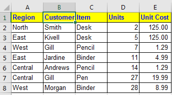
All of these might be confusing to understand. Let's understand how to use the function using an example. Here we have this data:
And we have this query
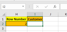
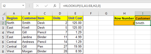
I want to retrieve data from table in I2 by just changing heading in I1 and row number in H2.
To do this, I write this HLOOKUP formula in cell I2
| =HLOOKUP(I1,A1:E8,H2,0) |
Now whenever you change heading, the HLOOKUP formula will show data of that heading.

The above HLOOKUP function will look for exact match in the first row of table and will return the value from given row number.
If you want an approximate match use 1 instead of 0 at range_lookup.
Pro Notes:
|
HLOOKUP is very useful if you are searching for data row wise. It can be combined with INDEX function to get data using headings row titles.
The HLOOKUP function is available in Excel 2016, 2013, 2010 and 2007 and may be in older versions too (I never used them).
You can also perform lookup exact matches using INDEX and MATCH function in Excel. Learn more about How to do Case Sensitive Lookup using INDEX & MATCH function in Excel. You can also look up for the partial matches using the wildcards in Excel.
Here are all the observational notes using the HLOOKUP function in Excel
Notes :
Hope this article about How to use the HLOOKUP function in Excel is explanatory. Find more articles on finding and matching values in table and related Excel formulas here. If you liked our blogs, share it with your friends on Facebook. And also you can follow us on Twitter and Facebook. We would love to hear from you, do let us know how we can improve, complement or innovate our work and make it better for you. Write to us at info@exceltip.com.
Related Articles :
Use INDEX and MATCH to Lookup Value : The INDEX & MATCH formula is used to lookup dynamically and precisely a value in a given table. This is an alternative to the VLOOKUP function and it overcomes the shortcomings of the VLOOKUP function.
Use VLOOKUP from Two or More Lookup Tables : To lookup from multiple tables we can take an IFERROR approach. To lookup from multiple tables, it takes the error as a switch for the next table. Another method can be an If approach.
How to do Case Sensitive Lookup in Excel : The excel's VLOOKUP function isn’t case sensitive and it will return the first matched value from the list. INDEX-MATCH is no exception but it can be modified to make it case sensitive.
Lookup Frequently Appearing Text with Criteria in Excel : The lookup most frequently appears in text in a range we use the INDEX-MATCH with MODE function.
Popular Articles :
How to use the IF Function in Excel : The IF statement in Excel checks the condition and returns a specific value if the condition is TRUE or returns another specific value if FALSE.
How to use the VLOOKUP Function in Excel : This is one of the most used and popular functions of excel that is used to lookup value from different ranges and sheets.
How to use the SUMIF Function in Excel : This is another dashboard essential function. This helps you sum up values on specific conditions.
How to use the COUNTIF Function in Excel : Count values with conditions using this amazing function. You don't need to filter your data to count specific values. Countif function is essential to prepare your dashboard.
The applications/code on this site are distributed as is and without warranties or liability. In no event shall the owner of the copyrights, or the authors of the applications/code be liable for any loss of profit, any problems or any damage resulting from the use or evaluation of the applications/code.


