
If you are trying to maintain sum debit and credit records in excel, you would probably want to have an automated balance column that will calculate the running balance. In this article, we will create ledger in excel with formula. This will keep a running balance in excel.

Well, it can be done easily by simple addition and subtraction.
The running balance is equal to the current balance + credit - debit.
If we formulate it for excel, the generic formula will be:
Balance: It is the current balance.
Credit: any income.
Debit: any withdrawal.
Let’s see an example.
Here I have this debit-credit data as an excel balance sheet. It has an opening balance of 15000.
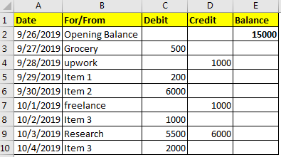
We need to have an running balance that will calculate the balance sheet each day.
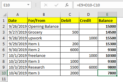
We have the opening balance in E2. write this formula in E3.
Drag it down. You have your ledger ready. Just copy above formula from above cell, whenever you make a new entry.
How it works?
Well it is an easy mathematics. We take the last balance, add anything credited and subtract whatever is debited. There is nothing much to explain here.
Handle Blank Entries
Now let’s say you have multiple dates update but the entries are yet to be updated. In that case, you would want to show a blank cell. We will check for the column cell if it is blank or not. If it's blank, there should be no entry in debit, credit and eventually in balance.
Write this formula in E2 and drag it down the cells.
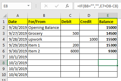
As you can see in the image above, we have balance shown only if there’s an entry.
You can set the check as per you requirement.
So yeah guys, this how you can have a excel check register. Let me know if you have any specific requirement in the comments section below.
Related Articles
Calculate Profit margin percentage
Simple interest formula in Excel
How to Use Compound Interest Function in Excel
Popular Articles:
The applications/code on this site are distributed as is and without warranties or liability. In no event shall the owner of the copyrights, or the authors of the applications/code be liable for any loss of profit, any problems or any damage resulting from the use or evaluation of the applications/code.


