
If you are in the transport business or import-export business then you know that shipping cost calculations is an important part of the business. And most of the time you have different shipping costs for different ranges of weights. So in this article, we will learn how to calculate shipping costs for given weight using VLOOKUP instead of multiple IFs.
Generic Formula for Shipping Cost Calculation
| =VLOOKUP(weight,sorted_cost_list,cost_per_Kg_Col,1)*weight |
Weight: It is the weight of which you want to calculate shipping cost.
Sorted_Cost_List: It is the table that contains the cost weights. The first column should be weight, sorted in ascending order.
Cost_per_Kg_Col: It is the column number that contains the cost per kg (or your unit) for shipping.
We will be using an approximate match which is why we are using 1 as the match type.
Let’s see an example to make things clear.
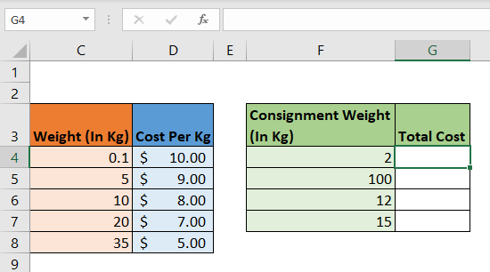
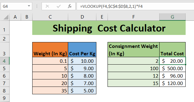
So here we have a sorted list of cost of freight by weight. The list is sorted in ascending order by weight. The cost of shipping is $10 if weight is less than 5 kg. If Weight is less than 10 kg then the cost is $9. And so on. If the weight is 35 kg or above the shipping cost per kg is $5.
We have a list of consignments that we need to ship. The weight is mentioned in the F column. We need to calculate the total cost for each shipment in the G column.
Let's use the above mentioned generic formula:
| =VLOOKUP(F4,$C$4:$D$8,2,1)*F4 |
Copy this formula down. And you have the total freight cost calculated in an instant. You can use it as the shipping cost calculator too. Just change the value in weight cells and the cost of the weight will be displayed.
How does it work?
We are using an approximate match of VLOOKUP to calculate the cost that needs to be applied on a given weight.
In the example above, we look for 2 in the table. VLOOKUP searches upside down. First it checks 0.1. It moves to next and finds the next value 5. Since 5 is greater than 2, VLOOKUP steps back and picks 0.1 as a match and returns a cost of 0.1 which is $10. Finally this cost is multiplied by the weight of consignment, which is 2 here and we get $20.
The step by step calculation looks like this:
| =VLOOKUP(F4,$C$4:$D$8,2,1)*F4 |
| =VLOOKUP(2,$C$4:$D$8,2,1)*2 |
| =10*2 |
| =20 |
A nested IF equivalent would look something like this,
| =IF(F4>=35,5,IF(F4>=20,7,IF(F4>=10,8,IF(F4>=5,9,10))))*F4 |
Isn't it too lengthy. Imagine if you had 100 intervals, then using a nested IF will not be a smart option. Using a VLOOKUP in such a conditional calculation is better than IF and IFS.
Here we are calculating shipping costs by weight. Similarly, you can calculate shipping costs by miles or other constraints.
So yeah guys, this is how you can calculate shipping costs in Excel easily. I hope this blog helped you. If you have any doubts or special requirements, ask me in the comments section below. I'll be happy to answer any Excel/VBA related questions. Till then keep learning, keep Excelling.
Related Articles:
How to Retrieve Latest Price in Excel | It is common to update prices in any business and using the latest prices for any purchase or sales is a must. To retrieve the latest price from a list in Excel we use the LOOKUP function. The LOOKUP function fetches the latest price.
VLOOKUP function to calculate grade in Excel | To calculate grades IF and IFS are not the only functions that you can use. The VLOOKUP is more efficient and dynamic for such conditional calculations.To calculate grades using VLOOKUP we can use this formula...
17 Things About Excel VLOOKUP | VLOOKUP is most commonly used for retrieving matched values but VLOOKUP can do a lot more than this. Here are 17 things about VLOOKUP that you should know to use effectively.
LOOKUP the First Text from a List in Excel | The VLOOKUP function works fine with wildcard characters. We can use this to extract the first text value from a given list in excel. Here is the generic formula.
LOOKUP date with last value in list | To retrieve the date that contains the last value we use the LOOKUP function. This function checks for the cell that contains the last value in a vector and then uses that reference to return the date.
How to Lookup Multiple Instances of a Value in Excel : To retrieve multiple stances of a matched value from a range we can use INDEX-MATCH with SMALL and ROW functions together. This makes up a complex and huge formula but gets the work done.
Popular Articles:
50 Excel Shortcuts to Increase Your Productivity | Get faster at your task. These 50 shortcuts will make you work even faster on Excel.
How to use Excel VLOOKUP Function| This is one of the most used and popular functions of excel that is used to lookup value from different ranges and sheets.
How to use the Excel COUNTIF Function| Count values with conditions using this amazing function. You don't need to filter your data to count specific values. Countif function is essential to prepare your dashboard.
How to Use SUMIF Function in Excel | This is another dashboard essential function. This helps you sum up values on specific conditions.
The applications/code on this site are distributed as is and without warranties or liability. In no event shall the owner of the copyrights, or the authors of the applications/code be liable for any loss of profit, any problems or any damage resulting from the use or evaluation of the applications/code.


