
In this article, we will learn How to Hide the Display of Zero Values in Excel.
Scenario:
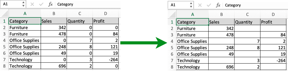
Problem here is working with excel data, sometimes we need to treat 0 as a blank cell. For example getting to know the average time spent on work each day. Now you think why it is a problem as the average function gives different results for data with 0 values and same data with blank cells. Another example can be printing out a data page with blank cells, no zero values. This happens because zero in excel is a number not a blank cell. So to avoid zeroes in your data use one of mentioned methods depending upon your usage. Not every method can be used for each purpose as in some methods zero is made invisible. So make your choice the right way.
First way : Custom format
Select the whole table and Go to Format cells Dialog box by going to Home tab, click Format > Format Cells or just using Ctrl + 1 keyboard shortcut. Then Go to Custom type 0;-0;;@ and click Ok.

You can get back zeroes by switching it back to General.
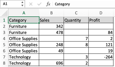
As you can see from the snapshot, This will make the data have more meaning than with zero values. This method is easy and convenient and is the common practice.
Second way : using Advanced Options
Another way using the Excel Advanced options. To make changes to the whole sheet and needed that change for later purpose. So go to File > Options > Advanced. And
Under Display options for this worksheet, select a worksheet, and then do one of the following:
To display zero (0) values as blank cells, uncheck the Show a zero in cells that have zero value check box.
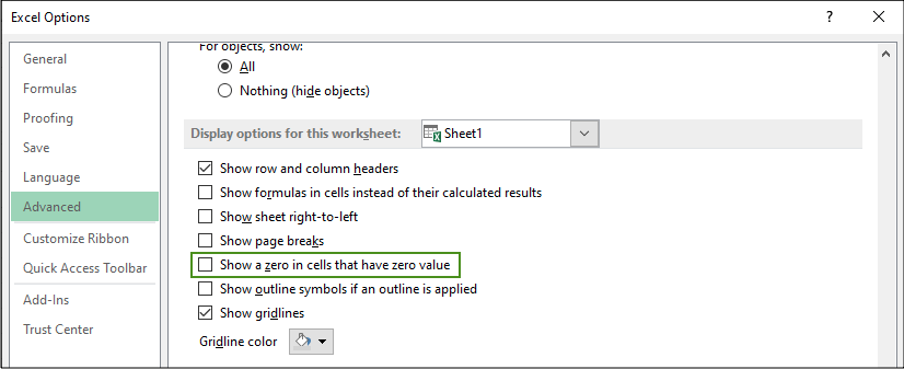
To display zero (0) values back in cells, check the Show a zero in cells that have zero value check box. As you can see from the snapshot, This will make the data have more meaning than with zero values.
Third way : using IF function
It's the space consuming way but very effective for calculation with functions like AVERAGE function which considers blank cells and zero (0) values differently.
Use the Formula for the first cell, =IF(cell_ref=0, "", cell_ref) And then copy the formula to all other cells to get the data with blank cells. Now you can use this data wherever you need either for calculation or printing.
Fourth way : Using Conditional formatting
This is the way to make zero (0) invisible with the background data, so zero values in the table don't get printed. Generally the excel cell background is White. So you can either change the background color to the same color of font or vice-versa. Here we select the data and Go to Conditional Formatting > Highlight Cells Rules > Equal To.
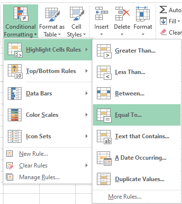
This will open up the Equal to value box.

In the box on the left, type value as 0 and In the box on the right, select Custom Format. It will open up the Format Cells box.
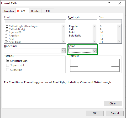
Click the Font tab as shown in above snapshot .In the Color box, select white, and then click OK. Or switch it to whatever background color you are working on.
Here are all the observational notes using the formula in Excel
Notes :
Hope this article about How to Hide the Display of Zero Values in Excel is explanatory. Find more articles on calculating values and related Excel formulas here. If you liked our blogs, share it with your friends on Facebook. And also you can follow us on Twitter and Facebook. We would love to hear from you, do let us know how we can improve, complement or innovate our work and make it better for you. Write to us at info@exceltip.com.
Related Articles :
Ignore zero in the Average of numbers : calculate the average of numbers in the array ignoring zeros using AVERAGEIF function in Excel.
How to Convert date to text in Excel : In this article we learned how to convert text into date, but how do you convert an excel date into text. To convert an excel date into text we have a few techniques.
How To Highlight Cells Above and Below Average Value : highlight values which are above or below the average value using the conditional formatting in Excel.
Calculate Weighted Average : find the average of values having different weight using SUMPRODUCT function in Excel.
Average Difference between lists : calculate the difference in average of two different lists. Learn more about how to calculate average using basic mathematical average formula.
Average numbers if not blank in Excel : extract average of values if cell is not blank in excel.
AVERAGE of top 3 scores in a list in excel : Find the average of numbers with criteria as highest 3 numbers from the list in Excel.
Popular Articles :
How to use the IF Function in Excel : The IF statement in Excel checks the condition and returns a specific value if the condition is TRUE or returns another specific value if FALSE.
How to use the VLOOKUP Function in Excel : This is one of the most used and popular functions of excel that is used to lookup value from different ranges and sheets.
How to use the SUMIF Function in Excel : This is another dashboard essential function. This helps you sum up values on specific conditions.
How to use the COUNTIF Function in Excel : Count values with conditions using this amazing function. You don't need to filter your data to count specific values. Countif function is essential to prepare your dashboard.
The applications/code on this site are distributed as is and without warranties or liability. In no event shall the owner of the copyrights, or the authors of the applications/code be liable for any loss of profit, any problems or any damage resulting from the use or evaluation of the applications/code.


My worksheet hides all zeros that are supposed to be hidden except for one cell (although there are also a few cells that reflect zero that are intended to reflect zero). Because there are some cells in the worksheet that are intended to reflect 0.00, I cannot use the "Display Options" method to hide zeros. All cells that are intended to have hidden zeros have been custom formatted as: 0.00;-0.00;;@, but the one defiant cell still reflects a visible 0.00. Other cells in the same column and row do not do this. The formulas in the cells immediately adjacent to (and including) the delinquent cell are all correct, so it has to be something with the formatting. I have tried changing the custom formatting for that cell to: 0;-0;;@ as well as ;;; but the cell still reflects a visible 0.00. I have also tried conditionally formatting that individual cell to change the font to the background color for the cell (white) if the cell value equals 0, but it STILL reflects a visible (black) 0.00.
The cell is AF20. The formula is =IF(AND(I200,AS19>8-I20,AI20=0,AL20=0,AM20=0),8-I20,IF(AND(I20<=8,AS19<8-I20,AI20=0,AL20=0,AM20=0),AS19,0)). I am an excel novice and I'm out of ideas. I have tried researching solutions, but the only solutions I have found are things I have already tried. Any suggestions?
Hey APSmith,
I think I understood your issue. Conditional formatting is not the solution to your problem. The problem lays in the custom formatting cell option. Use the character wisely checking the keyboard settings before typing. But it's not a worrying thing. Try the Custom formatting option again. Excel may sometimes surprise you with its tricky results. Do let us know more about the problem after trying again.
Thanks
can we do this via keyboard (Any Shortcut)
Thank You for the tutorial!
I used the "Custom" 0;-0;;@ but it now rounds my number to the nearest whole. I need the decimals. How do I do that?
Hi Paul,
Can you please tell us exactly what you are trying to enter in the cell. So that we can assist you accordingly.
Thanks,
Site Admin
I have a spreadsheet with multiple columns, specifically I am dealing with species of plants. The last column in the sheet gives the overall % each species occupies out of 100%. How do I leave the cells formatted and prevent 0% from showing up. The table is too confusing with all the 0%'s and it is not necessary for me to show 0%. Thanks for your time