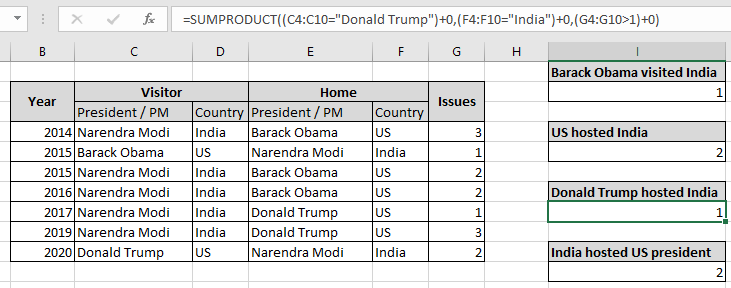
In this article, we will learn Count multiple ranges with one criteria in microsoft excel.
Scenario:
In simple words, while working with data tables, sometimes we need to count the cells where more than two ranges meet criteria. In Excel, You can perform tasks like operations over multiple ranges using the formula explained below. Criteria can be applied over text, number or any partial match in Excel. Criteria inside the formula executed using the operators. Operators like equals to ( = ), less than equal to ( <= ), greater than ( > ) or not equals to ( <> ).
How to solve the problem?
For this problem, we will be required to use the SUMPRODUCT function. Now we will make a formula out of the function. Here we are given two ranges of data and we need to count the rows that meet 3 criterias. SUMPRODUCT function returns the SUM of corresponding TRUE values (as 1) and ignores values corresponding to FALSE values (as 0) in the returned array
Generic formula:
| = SUMPRODUCT ( ( rng_1 op_1 crit_1 ) + 0 , ( rng_2 op_2 crit_1 ) + 0 , rng_2 op_2 crit_1 ) + 0 ) |
rng : range to look for
crit : criteria to apply
op : criteria operator, condition given as operator between range & criteria
+0 : converts boolean values to binary(0 & 1).
Example:
All of these might be confusing to understand. So, let's test this formula via running it on the example shown below. Here we need to find the count of rows listed in range having 3 conditions. Here we have a list of diplomat meetings held between India & US from 2014. The table shows the President / PM with the country label and year. The table is also divided in parts representing home country and the visiting country list.
Conditions listed below:
US president "Barack Obama visited India having issues less than 2.
Use the Formula:
| = SUMPRODUCT ( ( C4:C10 = "Barack Obama" ) + 0 , ( F4:F10 = "India" ) + 0 , ( G4:G10 < 2 ) + 0 ) ) |
C4:C10="Barack Obama" : President matching "Barack Obama" in the visiting list.
F4:F10="India" : host country matching "India".
G4:G10<2 : issues less than two.
+0 : converts boolean values to binary(0 & 1).
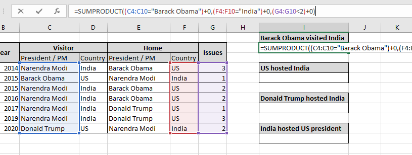
Here the range is given as cell reference. Press Enter to get the count.
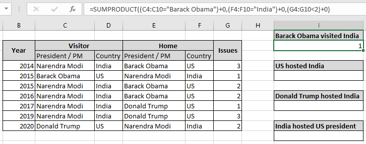
As you can see, only one time US president Barack Obama visited India which happened in 2015. This shows that the formula extracts the count of times matched in the corresponding array. As there is also one and same time when the US president "Barack Obama" visited India where issues is also equals to 1 which is less than 2.
With equals to Criterias:
The above example was easy. So to make it interesting we will count how many times US hosted India starting from 2014 as by data.
Conditions listed below:
US hosted India having issues is equal to 2.
Use the Formula:
| =SUMPRODUCT ( ( F4:F10 = "US" ) + 0 , ( D4:D10 = "India" ) + 0 , ( G4:G10 = 2 ) + 0 ) |
F4:F10="US" : host country matching "US".
D4:D10="India" : visiting country matching "India".
G4:G10=2 : issues equals to two.
+0 : converts boolean values to binary(0 & 1).
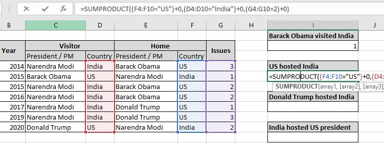
Here the range is given as cell reference. Press Enter to get the count.
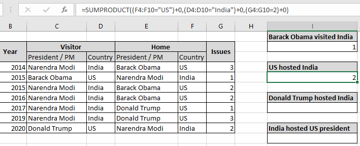
As you can see, there are 2 times where the US hosted India and issues equals to two. This shows that the formula extracts the count of times matched in the corresponding array. As there are 5 times when the US hosted India but issues were either 1 or 3, But here we need issues to be matched with 2.
With greater than Criterias:
Here to make it interesting we will count how many times US president "Donald Trump" hosted Indian Prime minister starting from 2014 as by data.
Conditions listed below:
US president "Donald Trump" hosted India having issues is greater than 1.
Use the Formula:
| =SUMPRODUCT ( ( C4:C10 = "Donald Trump" ) + 0 , ( F4 : F10 = "India" ) + 0 , ( G4:G10 >1 ) + 0 ) |
F4:F10="US" : host president matching "Donald Trump".
D4:D10="India" : visiting country matching "India".
G4:G10=2 : issues equals to two.
+0 : converts boolean values to binary(0 & 1).
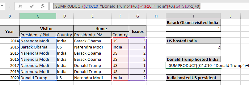
Here the range is given as cell reference. Press Enter to get the count.
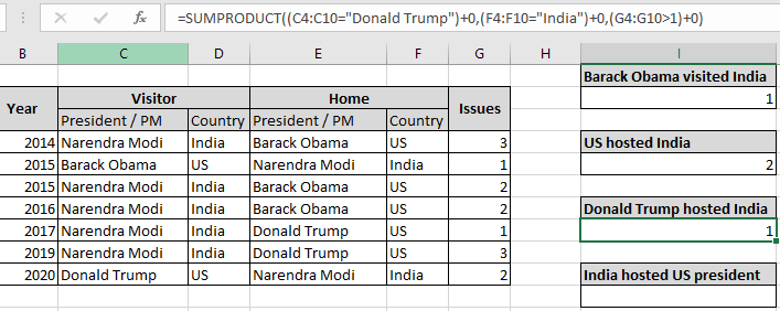
As you can see, one time where the US president "Donald Trump" hosted India and issues greater than two. This shows that the formula extracts the count of times matched in the corresponding array. As there are 2 times when the US president "Donald Trump" hosted India but issues were either 1 or 3, But here we need issues to be greater than 1 which is 3 lies in year 2019.
With issues not considered in Criteria:
Here to make it easy and convenient to understand, we will count how many times in total the US president visited India starting from 2014 as by data.
Conditions listed below:
The US president visited India in total from 2014.
Use the Formula:
| =SUMPRODUCT((F4:F10="India")+0,(D4:D10="US")+0) |
F4:F10="US" : host country matching "US".
D4:D10="India" : visiting country matching "India".
G4:G10=2 : issues equals to two.
+0 : converts boolean values to binary(0 & 1).
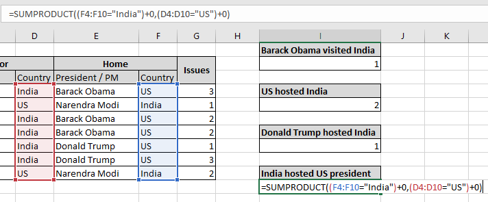
Here the range is given as cell reference. Press Enter to get the count.
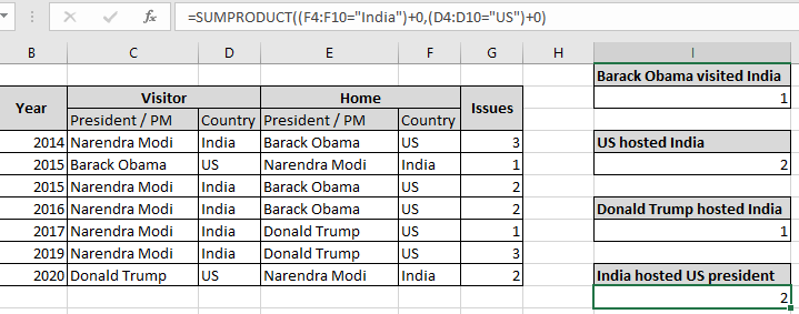
As you can see, 2 times where the US visited India and issues greater than two. This shows that the formula extracts the count of times matched in the corresponding array. As there was one time when the US president "Barack Obama" visited India in 2015 and one time when the US president "Donald Trump" visited India in the year 2020.
You can also perform ranges as criteria. Count the cells where 2 ranges meet criteria. Learn more about Countif with SUMPRODUCT in Excel here.
Here are some observational notes shown below.
Notes:
Hope this article about Count multiple ranges with one criteria in microsoft excel is explanatory. Find more articles on calculating values and related Excel formulas here. If you liked our blogs, share it with your friends on Facebook. And also you can follow us on Twitter and Facebook. We would love to hear from you, do let us know how we can improve, complement or innovate our work and make it better for you. Write to us at info@exceltip.com.
Related Articles :
How to use the COUNTIF Function in Excel : Count values with conditions using this amazing function. You don't need to filter your data to count specific values. Countif function is essential to prepare your dashboard.
How to use the SUMPRODUCT function in Excel: Returns the SUM after multiplication of values in multiple arrays in excel.
COUNTIFS with Dynamic Criteria Range : Count cells selecting the criteria from the list of options in criteria cell in Excel using data validation tool.
COUNTIFS Two Criteria Match : multiple criteria match in different lists in table using the COUNTIFS function in Excel
COUNTIFS With OR For Multiple Criteria : match two or more names in the same list using the OR criteria applied on the list in Excel.
How to Use Countif in VBA in Microsoft Excel : Count cells with criteria using Visual Basic for Applications code in Excel macros.
How to use wildcards in excel : Count cells matching phrases in text lists using the wildcards ( * , ? , ~ )in excel
Popular Articles :
How to use the IF Function in Excel : The IF statement in Excel checks the condition and returns a specific value if the condition is TRUE or returns another specific value if FALSE.
How to use the VLOOKUP Function in Excel : This is one of the most used and popular functions of excel that is used to lookup value from different ranges and sheets.
How to Use SUMIF Function in Excel : This is another dashboard essential function. This helps you sum up values on specific conditions.
How to use the COUNTIF Function in Excel : Count values with conditions using this amazing function. You don't need to filter your data to count specific values. Countif function is essential to prepare your dashboard.
The applications/code on this site are distributed as is and without warranties or liability. In no event shall the owner of the copyrights, or the authors of the applications/code be liable for any loss of profit, any problems or any damage resulting from the use or evaluation of the applications/code.