To find sum of numbers based on criteria, we can use a combination of SUM, MATCH, COUNTIF & OFFSET functions to retrieve the output.
SUM: Adds all the numbers in a range of cells
Syntax: =SUM(number1,number2,...)
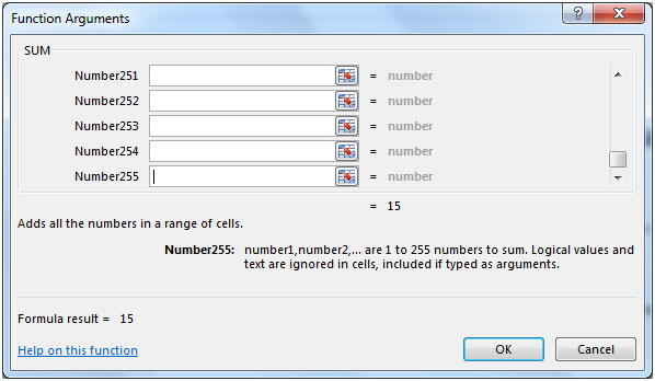
There can be maximum 255 arguments. Refer below shown screenshot:

MATCH function searches for a specified item in a selected range of cells, and then returns the relative position of that item in the range.
Syntax =MATCH(lookup_value,lookup_array,match_type)
COUNTIF: Counts the number of cells within a range that meets the condition.
Syntax: =COUNTIF(range,criteria)
OFFSET: Returns a reference to a range that is a given number of rows and columns from a given reference.
Syntax: =OFFSET(reference,rows,cols,height,width)
reference: It is a reference to a cell or range of cells from which the offset will be applied.
rows: The number of rows up or down that you want to apply as the offset to the range.
cols: The number of columns left or right that you want to apply as the offset to the range.
height: This is optional. It is the number of rows that you want the returned reference to be.
width: This is optional. It is the number of columns that you want the returned reference to be.
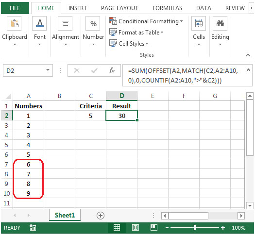
Let us take an example:
Column A contains an ascending list of numbers. We need a formula that will sum up all the numbers in column A larger than 2 which is our criterion in cell C2.


The applications/code on this site are distributed as is and without warranties or liability. In no event shall the owner of the copyrights, or the authors of the applications/code be liable for any loss of profit, any problems or any damage resulting from the use or evaluation of the applications/code.
How to get the sum of values with multiple values in criteria column.
For Eg: I want the sum of all the values which are equal to the list in column C "Criteria"
And Criteria will have 2, 5, 6 and 7
You can do this using curly braces when defining criteria.
=SUMIF(C:C,{2,5,6,7}, sum_range). Use CTRL+SHIFT+Enter once you have written the formula.Or you can use the sumproduct function to do so. Here I have explained it. https://www.exceltip.com/summing/sum-if-with-sumproduct-and-or-criteria-in-excel.html