

In this article, we will learn How to Sum Values In a Range Specified By Indirect Cell References in Excel.
Sum values in specific part of range
Cell reference and array reference is the most common usage for an excel user. It means picking up the value using the cell address so as to just change the value in the cell to get the new result. For example if you need to find the sum of the first 20 numbers in column A, you would use =SUM(A1:A120) . Now if you need for next 20. You have to edit the whole formula. Now you know the INDIRECT function which will help you understand the efficient use excel formula.
SUM formula in Excel
| =SUM( INDIRECT ( "A"&B1&":A"&B2 ) |
Explanation:
Example :
All of these might be confusing to understand. Let's first understand how to use the INDIRECT function using an example.
Here If value in cell B1 contains 500, A1 contains D1 & we use INDIRECT function in D1 cell =INDIRECT(B1), then result would be 500

So the function returns the value in the D1 cell which is 500.
Different usage
You can use it in many forms as shown here.
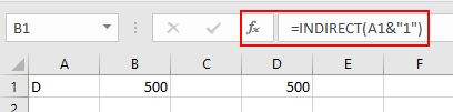
Here & operator is used for joining the text to get a full address of the cell. So A1 has D and 1 is added to D, get D1 cell ref.
You can directly refer to any cell.
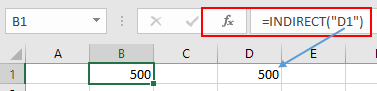
Here D1 is directly supplied to get the return from D1 address.
SUM values in range using INDIRECT function
You can use it with other functions to get the sum of the range given by cell reference. Here given a range from A1:A6. But we only need the sum from start(B1) to end (B2). Follow the below steps.
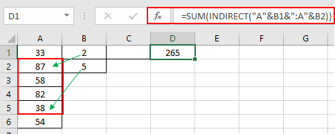
Here Range is provided to Sum functions referring to A2 : A5 range.
The above shown formula will add the sum of values as specified in column B. If we change the value in cell B2 from 3 to 4 then the formula will calculate the result accordingly.
Here are all the observational notes using the formula in Excel
Notes :
Hope this article about How to Sum Values In a Range Specified By Indirect Cell References in Excel is explanatory. Find more articles on calculating values and related Excel formulas here. If you liked our blogs, share it with your friends on Facebook. And also you can follow us on Twitter and Facebook. We would love to hear from you, do let us know how we can improve, complement or innovate our work and make it better for you. Write to us at info@exceltip.com.
Related Articles :
All About Excel Named Ranges : excel ranges that are tagged with names are easy to use in excel formulas. Learn all about it here.
The Name Box in Excel : Excel Name Box is nothing but a small display area on top left of excel sheet that shows the name of active cell or ranges in excel. You can rename a cell or array for references.
How to Get Sheet name of worksheet in Excel : CELL Function in Excel gets you the information regarding any worksheet like col, contents, filename, ..etc. Learn how to get the sheet name using the CELL function here.
How To Get Sequential Row Number in Excel : Sometimes we need to get a sequential row number in a table, it can be for a serial number or anything else. In this article, we will learn how to number rows in excel from the start of data.
Increment a number in a text string in excel : If you have a large list of items and you need to increase the last number of the text of the old text in excel, you will need help from the two TEXT and RIGHT functions.
Popular Articles :
How to use the IF Function in Excel : The IF statement in Excel checks the condition and returns a specific value if the condition is TRUE or returns another specific value if FALSE.
How to use the VLOOKUP Function in Excel : This is one of the most used and popular functions of excel that is used to lookup value from different ranges and sheets.
How to use the SUMIF Function in Excel : This is another dashboard essential function. This helps you sum up values on specific conditions.
How to use the COUNTIF Function in Excel : Count values with conditions using this amazing function. You don't need to filter your data to count specific values. Countif function is essential to prepare your dashboard.
The applications/code on this site are distributed as is and without warranties or liability. In no event shall the owner of the copyrights, or the authors of the applications/code be liable for any loss of profit, any problems or any damage resulting from the use or evaluation of the applications/code.


How to use this formula between 2 sheet.
If you want to sum from Sheet2 then use this formula.
=SUM(INDIRECT(“Sheet2!A”&B1&”:A”&B2))
where B1 and B2 can have any row number. If B1 has 2 than and B2 has 5 than range sheet2!B2:B5 will be summed up.
You can take help of this article too for summing across different sheet.
https://www.exceltip.com/summing/summing-values-from-cells-in-different-sheets.html
Good day,
I tried this formula in a workheet and the result I got was volatile. There are no blanks between the row range. What went wrong please?
Thank you
Above shows summing a column. Nice
How about summing a row?
If you have data numbers in A1:E1 and column letters (A and E) in A2 and A3 you want to sum in same fashion as above. use this formula
=SUM(INDIRECT(A2&"1:"&A3&"1"))
How can I change the offset starting reference so that it can change for every row in formula? For example,
E1=SUM(OFFSET(F1,0,0,1,52))
E2=SUM(OFFSET(F2,0,0,1,52))
E3=SUM(OFFSET(F3,0,0,1,52))
The starting reference will change automatically when you copy down your formula. This is called relative referencing and it is default in Excel Formulas.
You can read about it here: https://www.exceltip.com/excel-generals/relative-and-absolute-reference-in-excel.html