
In this article, we will learn how to find the maximal or minimal string, based on alphabetic order to retrieve the minimal or maximal values from a filtered list. We use the Subtotal function in Microsoft Excel 2010.
MATCH: The Match formula returns the cell number where the value is found in a horizontal or vertical range.
Syntax of “MATCH” function:=MATCH(lookup_value,lookup_array,[match_type])
INDEX: The Index formula returns a value from the intersection between the row number and the column number in an Array. There are 2 syntaxes for the “INDEX” function.
1st Syntax of “INDEX” function: =INDEX (array, row_num, [column_num])
2nd Syntax of “INDEX” function:=INDEX (reference, row_num, [column_num], [area_num])
MAX: This function is used to return the largest number in a set of values. It ignores logical values and text.
Syntax of “MAX” function: =MAX(number1, [number2],….)
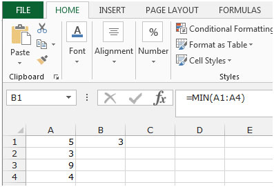
Example: Range A1:A4 contains the numbers. Now, we want to return the number that carries the maximum value.
Follow below given steps:-

MIN: This function is used to return the smallest number in a set of values. It ignores logical values and text.
Syntax of “MIN” function: =MIN(number1, [number2],….)
Example: Range A1:A4 contains a set of numbers. Now, we want to return the Minimum number.
Follow below given steps:-
COUNTIF: - We use this function to count the words. Using this function, we can easily find how many times one word is appearing.
The Syntax of “COUNTIF” function: =COUNTIF (Range, Criteria)
For Example: - Column A contains the Fruit list from which we want to count the number of Mango.
To count the number of Mango, follow below mention formula:-
=COUNTIF(A2:A6,"Mango"), and then press Enter on your keyboard.
The function will return the 3. It means Mango is repeating 3 times in column A.
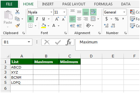
Let’s take an example to understand how we can find the minimum and maximum string based on alphabetic order.
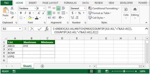
Maximum String based on alphabetic order
We have alphabet’s list in column A. To find the maximum string based on alphabetic order, follow the below given steps:-
Minimum String based on alphabetic order
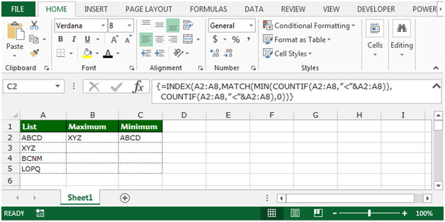
This is the way by which we can find the minimum and maximum string based on alphabets in Microsoft Excel.
The applications/code on this site are distributed as is and without warranties or liability. In no event shall the owner of the copyrights, or the authors of the applications/code be liable for any loss of profit, any problems or any damage resulting from the use or evaluation of the applications/code.


Hey,
I was wondering if there is a possibility, to simply ignore all text or blank cells and only search the maximum number value
(I would also need the formula to be able to evaluate a cell which has mixed contents, like: "V321-12")
Gotta say, great solution! It also led me to discover that a similar algorithm can be used to retrieve the data in one column that are associated with the maximum/minimum/etc. value of another column within a data table (for example, if I have a table of salespeople and individual sales, where each row is a single person's sales for that month, and I need to find who sold the most within a given month).
Kudos!
Thanks, you helped me a lot! I already found some other solutions for my problem, but all of them struggled on empty cells. Your solution exactly gives me what I want.
Does not work with c2:g2
Hi Tom,
Your question is not clear please describe you question.
Thanks
Excel Forum & Excel Tip's Team
The formula doesn't work because the quotation marks in this site are special characters that Excel doesn't know how to handle. If you copy and paste any formulas from here then you must replace the quotation marks with the generic basic ones you get from your keyboard.
The "Maximum String based on alphabetic order" formula presented here is pretty slow. A faster formula would be =INDEX(A2:A5,MATCH(0,COUNTIF(A2:A5,">"&A2:A5),0)) entered with ctrl-shift-enter since it is an array formula. However, if there are blank cells in the range that appear before the true maximum then it will just return 0, so if you need to allow for blank cells then use =INDEX(A2:A5,MATCH(0,IF(A2:A5"",COUNTIF(A2:A5,">"&A2:A5)),0)) with ctrl-shift-enter.
The formula presented in the article is better if you need to add extra constraints, though. For example =INDEX(A2:A5,MATCH(MAX(IF(A2:A5<"X",COUNTIF(A2:A5,”<”&A2:A5))),COUNTIF(A2:A5,”<”&A2:A5),0)) would find the maximum alphabetic string that starts with a character before "x"
The next example finds the maximum alphabetic string starting with a character before "x" and with a string length equal to the maximum string length of all of the strings starting with a character before "x". This is useful if your strings include numbers that you want treated as numbers so that for example "string10" is counted as being larger than "string9". This formula is entered with ctrl-shift-enter: =INDEX(A2:A5,MATCH(MAX(IF(A2:A5<"X",IF(LEN(A2:A5)=MAX(LEN(IF(A2:A5<"X",A2:A5))),COUNTIF(A2:A5,"<"&A2:A5)))),COUNTIF(A2:A5,"<"&A2:A5),0))
All of these array formulas run with a noticeable lag at around 1000 rows, so always limit them to as small a range as possible. Never just use entire columns as your ranges!
Ah, the site screwed up the formula for allowing for blank cells in the second paragraph of my comment. There is a less than sign immediately followed by a greater than sign which it removed because it treated them like a tag. It should have been:
=INDEX(A2:A5,MATCH(0,IF(A2:A5[less than][greater than]?”,COUNTIF(A2:A5,”>”&A2:A5)),0))
Just replace [less than] and [greater than] with their single character representations from the keyboard.
And it messed it up again! It added a question mark to the formula. There should be none.
Oh, the question mark should be a quotation mark.
I am trying to use the 'Maximum String based on alphabetic order' formula exactly as your instructions state, but it only returns the first value in the index range regardless of alphabetical value.