
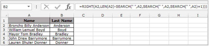
To extract the last word from the text in a cell we will use the “RIGHT” function with “SEARCH” & “LEN” function in Microsoft Excel 2010.
RIGHT:Return the last character(s) in a text string based on the number of characters specified.
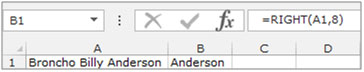
Syntax of “RIGHT” function: =RIGHT (text, [num_chars])
Example:Cell A1 contains the text “Broncho Billy Anderson”
=RIGHT (A1, 8), function will return “Anderson”
SEARCH:The SEARCH function returns the starting position of a text string which it locates from within the text string.
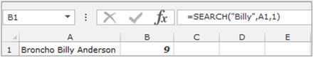
Syntax of “SEARCH” function: =SEARCH (find_text,within_text,[start_num])
Example:Cell A2 is containing the text “Broncho Billy Anderson”
=SEARCH ("Billy", A1, 1), function will return 9
LEN:Returns the number of characters in a text string.
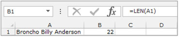
Syntax of “LEN” function: =LEN (text)
Example:Cell A1 contains the text “Broncho Billy Anderson”
=LEN (A1), function will return 22
Understanding the process of Extracting Characters from Text Using Text Formulas
Example 1: We have a list of Names in Column “A” and we need to pick the Last name from the list. We will use the “LEFT” function along with the “SEARCH” function.
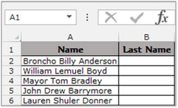
To separate the last word from a cell follow below steps:-
To Copy the formula to all the cells press key “CTRL + C” and select the cell B3 to B6 and press key “CTRL + V” on your keyboard.
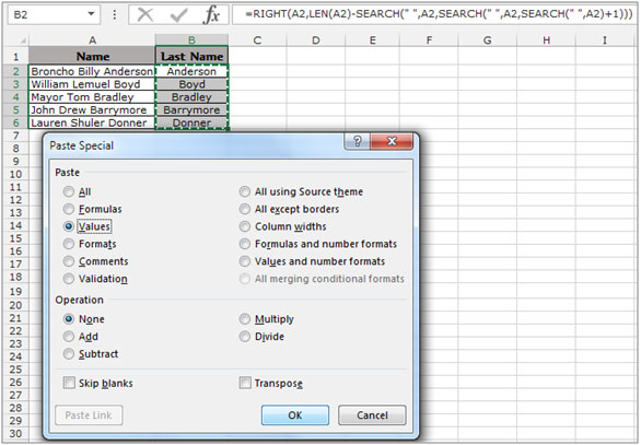
This is how we can extract the last word in a cell into another cell.
The applications/code on this site are distributed as is and without warranties or liability. In no event shall the owner of the copyrights, or the authors of the applications/code be liable for any loss of profit, any problems or any damage resulting from the use or evaluation of the applications/code.


How to separate One word from column ( common word in every Name on left)
Eg Here :- wanted to remove Total from every name
CUST_NAME
A K AGENCIES Total
A.K.ELECTRICALS Total
JAI DURGA ENTERPRISES Total
MURALI KRISHNA AGENCIES Total
GOYAL ILLUMINATIONZ Total
My column consists of the following data:
'1-5
'5-10
'3-8
'5-10
Is there an excel formula that can extract from the column the lowest range and the highest range? In this case '1-5 as the lowest and '5-10 as the highest range.
Hi Noble! As per your data sample, the largest will have the largest sum of lower bound and upper bound. For example, 5-10 will have a sum of 15. so using this you can get the largest or minimum range in the column.
To get sum of largest range use the below array formula. (I am assuming your data is in range A2:A5, after writing this, hit CTRL+SHIFT+ENTER.
=MAX(VALUE(LEFT(A2:A5,FIND("-",A2:A5)-1))+VALUE(RIGHT(A2:A5,LEN(A2:A5)-FIND("-",A2:A5))))
To get sum of lowest range use the below array formula. (I am assuming your data is in range A2:A5, after writing this, hit CTRL+SHIFT+ENTER.
=MIN(VALUE(LEFT(A2:A5,FIND("-",A2:A5)-1))+VALUE(RIGHT(A2:A5,LEN(A2:A5)-FIND("-",A2:A5)))).
I hope this will work for you.
The solution suggested here works only for 3 column data.
Imagine a list of Names from an address list with words separated by 1 or more spaces
Names can be very variable and some lines might be blank and some names might be one word only e.g.
J Smith
John S Doe
Mr & Mrs A B C Smithson
Harry
This formula will extract the last word in all the above cases.
"Smith", "Doe", "", "Smithson", "Harry"
=IF(ISERR(FIND(" ",A2)),IF(LEN(A2)=0,"",A2),RIGHT(A2,LEN(A2)-FIND("*",SUBSTITUTE(A2," ","*",LEN(A2)-LEN(SUBSTITUTE(A2," ",""))))))
Yes, one formula with SIX parentheses at the end!
The only spaces in the formula are between double quotes - there are 4 of them
It can be adapted to ignore empty lines or single word lines.
gs
Thank you. You saved me at least a half an hour of finding my own formula.
This is great!
How do you extract all names EXCEPT the last name?
Dan
Thanks a lot
love this
this is horrible.. but it actually works. so it is great! using that to sanitize badly maintained sheets before feeding it to automation.
thank you!
Thanks a ton! This saved me at least 5 lines of unnecessary code and 1 hour of brainstorming
Is there a way to extract the first and last letter of a word?
Sure can. Using the left and right described elsewhere and earlier. For example, the first letter is easy, if it's the first character, that is.
=LEFT(A1,1). - assuming your data is in A1
The last letter would be...
=RIGHT(A1,1)
Finally, you just concatenate these together ...
=LEFT(A1,1),RIGHT(A1,1)
Or
=CONCATENATE(LEFT(A1,1),RIGHT(A1,1))
"you might want to concatenate or 'join' those cells. if you're just working with text files, its quite easy.
example:
you have ""ARG12"" in A1, and "".gif"" in B1
=CONCATENATE(A1,B1)
this would result to: ""ARG12.gif""
if all those texts are on just TWO columns, you'd want to use this formula instead so that excel can have a reference point:
=CONCATENATE($A1,$B1)
hope this helps.
The Mace
"Greetings,
I am trying to see if there is a way to join two different colums of text into on colum? I am trying to populate my web store with these products from my distributor. One colum has the product name such a ARG12 and then the second colum has ""noimage.gif"" but I changed ""noimage.gif"" to just "".gif"" now if i could only find a way to merge or joing these two colums, then the image names would all be easily imported (there over 2000) and having to manually type a "".gif"" after each one would take forever...There must be a way to merge two colums of text? or a way to easily do this so that i end up with ARG12.gif in one colum?
Anyone?
Thanks,
Taylor reaume
An easier way to concatenate is just using the = sign.
=(cell)&(cell) ie =A2&B2
To include spaces or constants use "" around the value
=A2&" - "&B2
thanks for sharing another option to concatenate two cell,
really appreciated 🙂
Rishi Saw