
In this article we will learn how to apply conditional formatting in cell.
To apply Conditional formatting based on text, we use the Conditional Formatting option in Microsoft Excel.
Conditional Formatting: - It is used to highlight the important points with color in a report.
Let’s take an example and understand how we can apply formatting only to text containing cells.
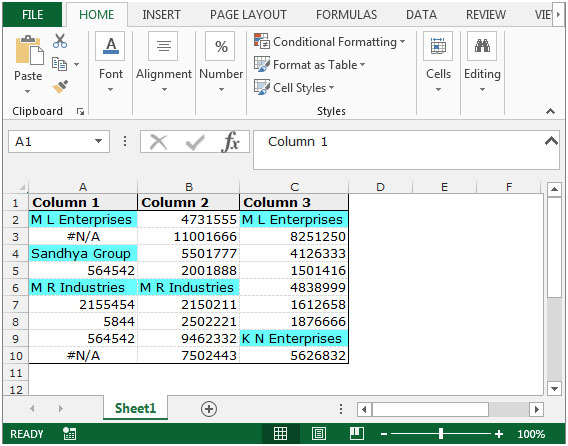
We have data in range A1:C10,in which Text and numbers are miscellaneous, from that we want to highlight the cells which is contain text.

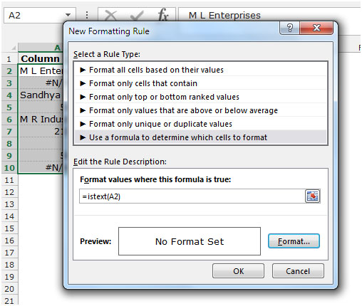
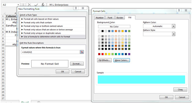
Follow below given steps to highlight the text contain cells:-
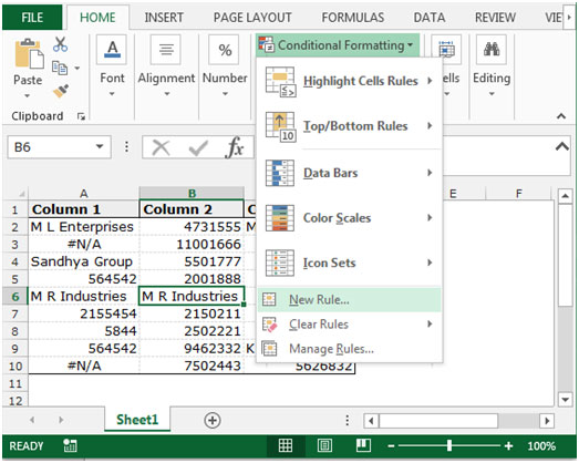
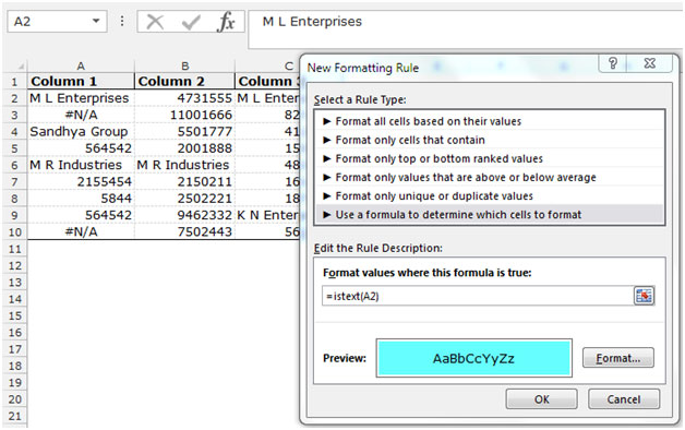
This is the way you can use conditional formatting for text containing cells in Microsoft Excel 2010 and 2013.
The applications/code on this site are distributed as is and without warranties or liability. In no event shall the owner of the copyrights, or the authors of the applications/code be liable for any loss of profit, any problems or any damage resulting from the use or evaluation of the applications/code.


Hi,
I am working with texts on excel but basically I would like to format the work by giving a number from 1 to 5. Basically, all the text cells containing the number 1 should be red. Number 2 yellow, number 3 orange and so on.
How can I condition this?
Thank you
Hi, I am looking for something quite apecifc
I want to
A) Make the a cell fill with colour if it has text in it
AND THEN
B) turn a specific colour based on what text is typed in the first column.
For example:
I want a Cell to go Green IF the row starts with 'John' AND that specific cell has text in it.
However, I want a cell that's row starts with 'Jack' to turn Red Aslong as it also has text in it too.
Hope you can help
Oli
if we enter a text in A1 & want to color B1 so what will be the string/syntax/method. Please reply...!!!
This article may help you.
https://www.exceltip.com/conditional-formatting/highlight-row-base-on-a-cell-value-in-excel.html
I have a question:
I have a cell string, that is formatted to turn red, if above or below two numbers. however, the sheet has a predetermined set of cells, and I would like to keep them from turning color unless something is written into the cells. So, I would like to keep the cell open, and clean unless something is written, then two conditional formats take place. BUT, I don't want to have to have my engineers expanding the spreadsheet. I want the formulas to exist in range already within the cells.
Right now, if I pull down formulas all cells are red in color simply because nothing is written in them, so by default, they are "BELOW" the cells conditional range. the top of the range is 2500, the bottom is 2000. So above 2500 and then below 2000 they should turn red, but not if the cell is void of text or number.
Hi Jeff,
This can be done easily by putting another conditional formatting for empty cells. This should be the first conditional formatting and set formatting to be the plan. Then put your conditional formatting and it will be done criteria.
This can be your schema
1) format plan IF ISBLANK(cell)
2) format red IF <2000
2) format red IF >2500
Hi,
I am looking for the rule of conditional formatting for text where are two words in the cell.
For example, If I look for one word the rule will be ( =ISTEXT(A1) ), But if I look for two words What will be the rule?
Thanks
If you want to highlight cells that have two words then use this formula in conditional formatting.
=COUNTIF(A2," ")=1
The logic is that two words must have 1 space. here we are counting spaces (" ") in A2. If there's only one space then it means it has two words hence it will fall TRUE, else FALSE.
If you want highlight cell if it has at least 2 words then use below formula.
=COUNTIF(A2," ")