
So, one day I was working on pivot report and I wanted to do some operation with pivot data. I started writing the formula and as I clicked on pivot field cell, I saw GETPIVOTDATA function there.
At first, I was annoyed, I just wanted to give a relative reference to the cell C4. So turned it off.
But later I understood the usefulness of the GETPIVOTDATA function of Excel. I understood when and how to use the GETPIVOTDATA function in Excel. So let's tear apart this GETPIVOTDATA function and see how it works.
You can write the GETPIVOTDATA function like any other function in Excel.
When in the dashboard you just want to get a dynamic update from the pivot table, GETPIVOTDATA really helps you to do so.
GETPIVOTDATA Function Syntax.
Data_Field: The field that you want to query from.
Pivot_table: A reference to any cell in a pivot table, so that formula knows which pivot table to use.
[field1, item1]: This is optional. But you’ll be using this more often. Rather than explaining it, I’ll show you…
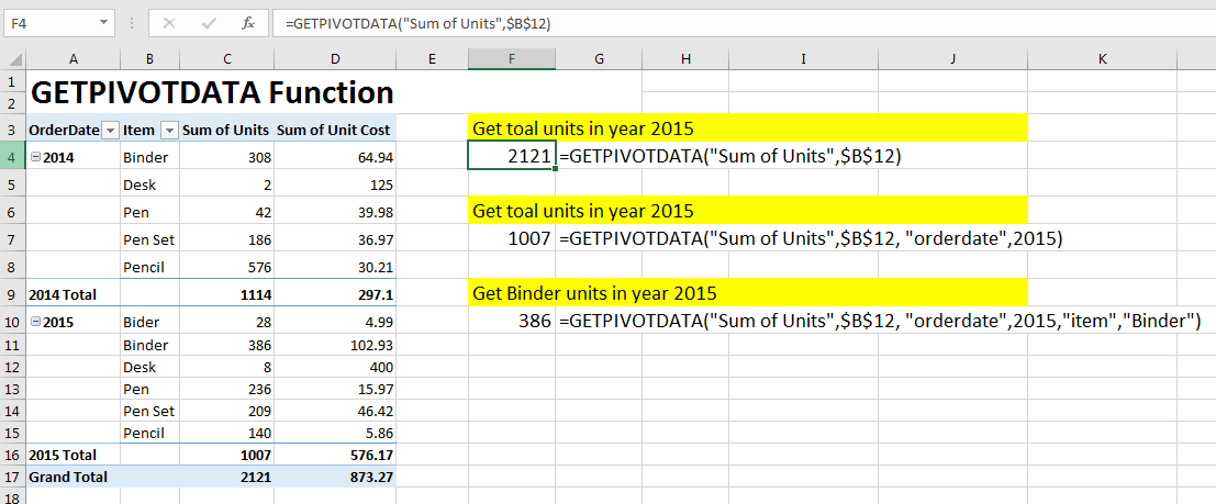
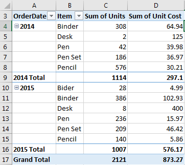
So, here we have this pivot table.
If, in a cell, I want to get a grand total of “Sum of Units” dynamically. Write this excel
GETPIVOTDATA formula.
This GETPIVOTDATA formula will return to 2121.
If you want to get a grand total of sum of unit cost, just replace "Sum of Units" with “sum of unit cost” and that will return 873.27. The reference $A$3 can be another reference as long as it is in the pivot table area. It is suggested to use the first cell since the pivot table never going to shrink to that level.
Let's see some more GETPIVOTDATA examples.
To get a total of “sum of units” in the year 2014, write this GETPIVOTDATA formula.
This will return to 1114. I assume that you know how to get a total of 2015.
To get the price of binder in the year 2015 write this GETPIVOTDATA formula.
So yeah guys, that's how you can excel GETPIVOTDATA function. In excel dashboards it can do magic. If you have any thought regarding this function or any other in Excel 2016 or older versions, mention it in the comments section below.
Related Articles:
Show hide field header in the pivot table
Popular Articles:
50 Excel Shortcuts to Increase Your Productivity
How to use the VLOOKUP Function in Excel
How to use the COUNTIF function in Excel 2016
How to Use SUMIF Function in Excel
The applications/code on this site are distributed as is and without warranties or liability. In no event shall the owner of the copyrights, or the authors of the applications/code be liable for any loss of profit, any problems or any damage resulting from the use or evaluation of the applications/code.


