
The number of items available for filtering is limited. Excel cannot filter columns in which the number of items exceeds 999 (not the number of rows).
To filter when there are more than 999 items, use advanced filter.
To create an advanced filter, we will use “OFFSET” and “COUNTA” functions in Microsoft Excel.
COUNTA: It returns the count of the number of cells which contain values.
Syntax of “COUNTA” function: =COUNTA (value1, value2, value3…….)
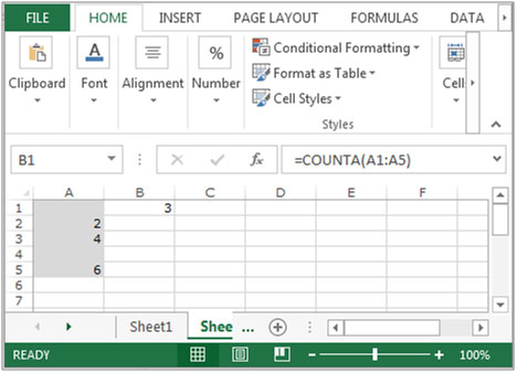
Example: In range A1:A5, cells A2, A3 and A5 contain the values, and cells A1and A4 are blank. Select the cell A6 and write the formula-
=COUNTA(A1:A5) the function will return 3
OFFSET: It returns a reference to a range that is offset a number of rows and columns from another range or cell.
Syntax of OFFSET function: =OFFSET (reference, rows, cols, height, width)
Reference:- This is the cell or range from which you want to offset.
Rows and Columns to move: - The number of rows you want to move from the starting point and both of these can be positive, negative or zero.
Height and Width: - This is the size of the range you want to return. This is an optional field.
Let’s take an example to understand the Offset function in Excel.
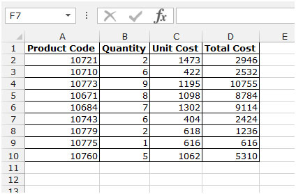
We have data in range A1:D10. Column A contains Product Code, Column B contains Quantity, column C contains per product cost and column D contains Total cost. We need to return the value of cell C5 in cell E2.
To get the desired outcome, we need to follow the below mentioned steps.

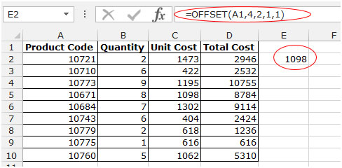
In this example, we need to obtain the value from the cell C5 to E2. Our reference cell is the first cell in the range which is A1 and C5 is 4 rows below and 2 columns to the right from A1. Hence, the formula is =OFFSET(A1,4,2,1,1) or =OFFSET(A1,4,2) (since 1,1 is optional).
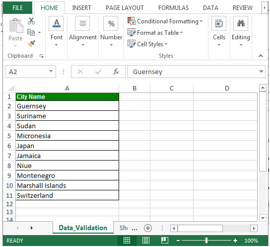
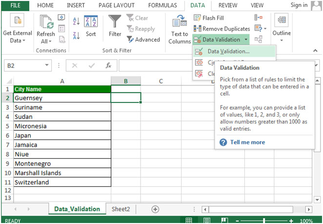
Now, let’s take an example to retrieve the last value in a dynamic list.
We have country names in a range. Now, if we add more countries to this list, it should be available in the drop down list automatically.
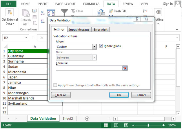
To prepare advanced filter, follow the below given steps:-
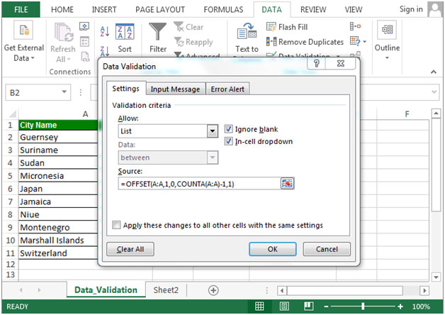
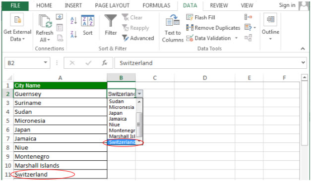
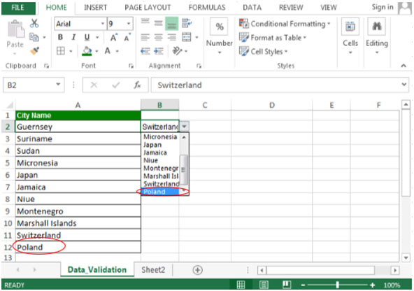
As soon as you add an entry in A12, it will be added to the dropdown list.
This is the way we can add more entries than 999 items in Microsoft Excel.
The applications/code on this site are distributed as is and without warranties or liability. In no event shall the owner of the copyrights, or the authors of the applications/code be liable for any loss of profit, any problems or any damage resulting from the use or evaluation of the applications/code.


