

In this article, we will learn How to format all worksheets in one go in Excel.
Scenario:
When working with multiple worksheets in Excel. Before proceeding to the analysis in excel, first we need to get the right format of cells. For example learning the products data of a super store having multiple sheets. For these problems we use the shortcut to do the task.
Ctrl + Click to select multiple sheets in Excel
To select multiple sheets at once. Go to excel sheet tabs and click all required sheets holding the Ctrl key.
Then format any of the selected sheets and the formatting done on the sheet will be copied to all. Only formatting not the data itself.
Example :
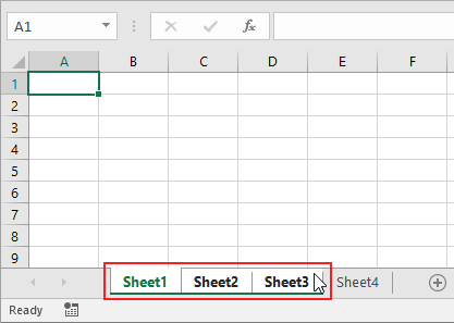
All of these might be confusing to understand. Let's understand how to use the function using an example. Here we have 4 worksheets and we need to edit the formatting of Sheet1 , Sheet2 and Sheet3.
For this we go step by step. First we go to the sheet tabs as shown below.

Select the Sheet1 and now select the Sheet2 with holding Ctrl key and then select Sheet3 keep holding the Ctrl key.
Now any format editing done on any of the selected three sheets will be copied to the other selected ones.
Here are all the observational notes using the formula in Excel.
Notes :
Hope this article about How to format all worksheets in one go in Excel is explanatory. Find more articles on calculating values and related Excel formulas here. If you liked our blogs, share it with your friends on Facebook. And also you can follow us on Twitter and Facebook. We would love to hear from you, do let us know how we can improve, complement or innovate our work and make it better for you. Write to us at info@exceltip.com.
Related Articles :
50 Excel Shortcuts to Increase Your Productivity : Get faster at your tasks in Excel. These shortcuts will help you increase your work efficiency in Excel.
Replace text from end of a string starting from variable position : To replace text from the end of the string, we use the REPLACE function. The REPLACE function use the position of text in the string to replace.
How to Select Entire Column and Row Using Keyboard Shortcuts in Excel : Selecting cells is a very common function in Excel. Use Ctrl + Space to select columns and Shift + Space to select rows in Excel.
How to Insert Row Shortcut in Excel : Use Ctrl + Shift + = to open the Insert dialog box where you can insert row, column or cells in Excel.
How to Select Entire Column and Row Using Keyboard Shortcuts in Excel : Use Ctrl + Space to select whole column and Shift + Space to select whole row using keyboard shortcut in Excel
Excel Shortcut Keys for Merge and Center : This Merge and Center shortcut helps you quickly merge and unmerge cells.
Excel REPLACE vs SUBSTITUTE function: The REPLACE and SUBSTITUTE functions are the most misunderstood functions. To find and replace a given text we use the SUBSTITUTE function. Where REPLACE is used to replace a number of characters in string…
Popular Articles :
How to use the IF Function in Excel : The IF statement in Excel checks the condition and returns a specific value if the condition is TRUE or returns another specific value if FALSE.
How to use the VLOOKUP Function in Excel : This is one of the most used and popular functions of excel that is used to lookup value from different ranges and sheets.
How to use the SUMIF Function in Excel : This is another dashboard essential function. This helps you sum up values on specific conditions.
How to use the COUNTIF Function in Excel : Count values with conditions using this amazing function. You don't need to filter your data to count specific values. Countif function is essential to prepare your dashboard.
The applications/code on this site are distributed as is and without warranties or liability. In no event shall the owner of the copyrights, or the authors of the applications/code be liable for any loss of profit, any problems or any damage resulting from the use or evaluation of the applications/code.


