
Consider a scenario, in which we are required to use helper column to get the output using VLOOKUP function. In this article, we will let you know how to get the output without using helper column by using the combination of VLOOKUP & CHOOSE functions.
Let’s take an example and understand:-
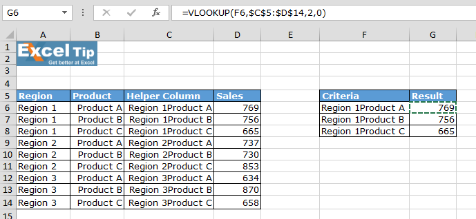
We have a sales report for 3 Region & 3 Products. In column E, there are criteria’s listed which are combination of Region & Product. We want a formula that will derive the result in column F by looking up value in column A, B & C.

The common way of getting the output is to use Helper column:
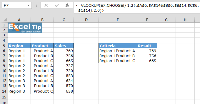
To get the output without using Helper column, use below given formula:-
Note:- This is an array formula which requires formula to be enclosed with curly brackets by using CTRL + SHIFT + ENTER.
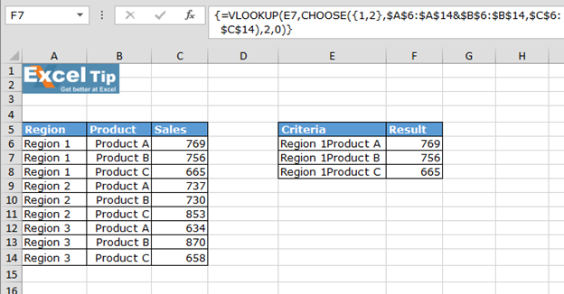
Hence, using Vlookup & Choose functions together we need not to use Helper column to find the result.
![]()
If you liked our blogs, share it with your friends on Facebook. And also you can follow us on Twitter and Facebook.
We would love to hear from you, do let us know how we can improve, complement or innovate our work and make it better for you. Write us at info@exceltip.com
The applications/code on this site are distributed as is and without warranties or liability. In no event shall the owner of the copyrights, or the authors of the applications/code be liable for any loss of profit, any problems or any damage resulting from the use or evaluation of the applications/code.


the formula is not giving the proper value