
So here we are, with calculations that give long decimal results.The value of PI is 3.14159265...god knows where it ends. But most of our work is done by just 3.14. This is called rounding. Let’s see how we can round the numbers in excel.
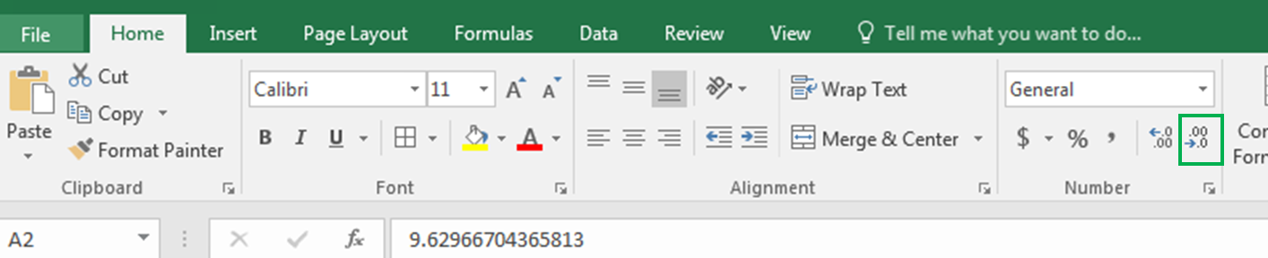
Let's say in cell A2 we have 92.45477919. To limit these decimal points you can go to Home Tab? Decrease Decimal and click it until you reach to your desired number of decimals.
Wouldn’t it be easy and time-saving if you can do it with a formula?
Excel provides three formulas for Rounding Numeric numbers:
| ROUND (value, num of decimal digits) | ROUNDUP(value, num of decimal digits) | ROUNDDOWN (value, num of decimal digits) |
Examples will make it easy.
The round function simply limits decimal value. It takes two arguments. First the value (the number that needs to be rounded) and second the number of decimals.
For example here in Cell A2, I have a random decimal number generated by RAND() function and then multiplied by 100. Now in Cell B2 I want to have only 1 decimal digit, so I write:
You can see the result in A2 in the below image.
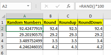
It shows only one digit.
Same as the ROUND function of Excel, the ROUNDUP function limits the decimal points shown but it always increases the last decimal digit by one.
This, too, takes two arguments. First the value (the number that needs to be rounded) and second the number of decimals.
Now in Cell C2, I want to have only 1 decimal digit but I want to increase it by one to compensate the leftover digits. So I write this formula in C2:

You can see that the value is rounded (92.5) to one decimal and it is increased by one.
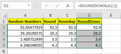
The ROUNDDOWN function just shows the last decimal digit as it is and makes all following decimal digits 0. In short, it prevents the rounding up of a number.
In Cell D2 I have written this formula:
You can see that 92.454779 is now 92.4. Similarly, all numbers in column D are shown as they depend on defined decimal digits.
Now you know how to harness control of these decimal digits to your desired number digits. I tried to explain ROUND functions in Excel in the most precise way. These Rounding functions are available in Excel 2016, 2013, 2010 and in older Excel versions.
Let me know if that would be helpful. If your problem is not solved then post it in the comments section.
The applications/code on this site are distributed as is and without warranties or liability. In no event shall the owner of the copyrights, or the authors of the applications/code be liable for any loss of profit, any problems or any damage resulting from the use or evaluation of the applications/code.


Hi. I have a formula like this =(($H2/50)*0.15)*100
How can I round it up?
Hi, Anne
if you want to round up the result to zero number of decimal points, use this formula.
Use ROUNDUP((($H2/50)*0.15)*100,0).
hi i have a problem. How do i get (1/3) to work in a "if " formula when the answer is only to be given in 3 digits
Hi, after rounded 3 CELLS 20.8 as 21 I got sum for these 3 CELLS is 62 not 63 similarly 20.2 ronded to 20 and sum of three is 61 not 60 how can I fix the problem
Hi, If you use ROUND or ROUNDUP Functions to round up values, the sum of these values will 63. But if you are using increasing or decreasing decimal point method for rounding up values, the sum will be shown of original values instead of sum of round up values.
Hi, I am trying to round ((M7)/(M9/100)^2) formula to the tenth, but it keeps giving me an error. How can I fix this?
Hello,
How would I get excel to continue to round up the highest fractions in a column until it hits a specific number then round down the remain.
Example:
C1: 9.43, C2: 9.78, C3: 8.6
I want excel to round the highest fractions first until it equals 28. Then round the remain down.
So since C3 is the highest it rounds to 9, c2 is the second it rounds to 10, c1 is not needed to round up as we have hit our total so it rounds down.
Then I want to capture the fractions that it rounded up or down so they offset next month.
Example carryover:
C1= .43, c2= -.22, c3= -.4
Thank you,
Craig
Hello,
How would I get excel to continue to round up the highest fractions in a column until it hits a specific number then round down the remain.
Example:
C1: 9.43, C2: 9.78, C3: 8.6
I want excel to round the highest fractions first until it equals 28. Then round the remain down.
So since C3 is the highest it rounds to 9, c2 is the second it rounds to 10, c1 is not needed to round up as we have hit our total so it rounds down.
Then I want to capture the fractions that it rounded up or down so they offset next month.
Example carryover:
C1=-.43, c2=-.22, c3=-.4
Thank you,
Craig
Hi,
Excel gives different results when I decrease decimel and when I use round function.
i.e
5,055 --> decrease decimel --> 5,05
5,055 --> round (or roundup) --> 5,06 (the correct one).
is this due to some Setting issue? how can i fix it?
thanks in advance
Hi Firat,
I thing the actual number would be something 5.0546... something and the default visible number would be 5.055 (default rounding). And when you round this number it will return 5.055
Hi
I have a formula that is date related as per the below, this calculates monthly budget lines but if the month is short by a day - ie: Nov it changes the budget line as it is calculating a 'short month' 0.9666667 instead of 1
do you know how I can round up the end formula whilst keeping the below
=(DATEDIF([@[Activity Start Date2]],[@[Activity Finish Date3]],"d"))/30
use ROUNDUP Function.
=ROUNDUP(DATEDIF([@[Activity Start Date2]],[@[Activity Finish Date3]],”d”))/30)
How do I use the roundup formula to a cell which already has a formula eg
cell A1 value = 60
cell A2 value = 8
cell A3 has a value =A1/A2. This leaves me a value of 7.5
I want to round off that value in cell A4. how would you write out the formula to achieve an 8 value
It is simple Bradley. Use Formula in A4 =ROUNDUP(A3,0)
I have the same question, but I want to nest the Round function inside the resulting cell. not create a new "Rounding" cell that references the formula cell.
In other words, I want the ROunding to be a part of the formula. So, in the result above, I want to round Cell A3 within itself.
As a caveat, the formula is an IF statement. Is this even possible?
Yes Keith. It is possible. Just write the formula as =ROUNDUP(A1/A2). Basically you just need to encapsulate the formula that will return a fractional result with the ROUNDUP function. The result will automatcally rounded up to specified decimal points.
my question is similar, but i'm using multiplication: =(B3*.1250). when i try to use ROUNDUP such as =ROUNDUP(B3*.1250) the error "you've entered too few arguments for this function" is returned. what needs to change?
You need to tell the number of decimal points you need. the roundup function takes two arguments. roundup(number, decimal_numbers). So B3*.1250 will return a number. Now if you want a whole number, you want zero decimals. Hence use this formula =ROUNDUP(B3*.1250,0). If you want 1 decimal point after whole number use =ROUNDUP(B3*.1250,1) and so on.
Hi all, I'm trying to round (to the nearest hundreth) the result of the sum of a range of numbers divided by another number.
Here's what I've attempted so far but it's not working (currently results in: #VALUE):
=ROUND(SUM(H7:V7/5280),2)
Any help would be greatly appreciated.
try this: =ROUND(SUM(H7:V7)/5280,-2)
you can use this article too https://www.exceltip.com/excel-format/using-the-round-function-to-round-numbers-to-thousands.html
Thanks William, it was what I was really looking for.
Thanks Alan. The formula does exactly what I need it to do. Perfect.
"The way I normally do this, is by dividing by 5, rounding to the nearest whole number, and then multiplying back by 5:
If the number you want to round in this way is in A1, then:
=ROUND(A1/5,0)*5
Does that solve your problem? "
I want to take my results for example, 213 and 212 and round up to 215 and round down to 210. I am trying to round up to "5" and down to "0". Does anyone know how to do this?