
In this article we will learn how to find the duplicate items in combined columns. To find duplicate items we use the “COUNTIF” and “IF” formulae in Microsoft Excel.
IF:-IF condition allows us to specify multiple conditions in a cell. It helps us to create the flexibility of the function in Microsoft Excel . Upto a maximum of 64 conditions can be placed inside an IF function.
Syntax of “IF” function: =if (logical test, [value_if_true], [value_if_false])
COUNTIFS: This function is used to return the count of same entry in the multiple range..
Syntax of “COUNTIFS” function: =COUNTIFS (Criteria_Range1, Criteria1,Criteria_Range2,Range2)
Let’s take an example and understand how we can find duplicate items in combined columns in Microsoft Excel.
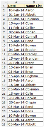
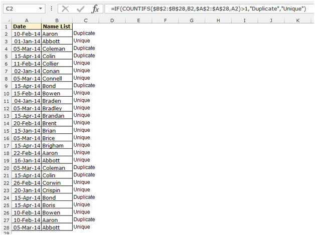
Example: - We have a list of names in range A2:A28, in which one name is entered many times. We need to find all the names which are entered more than once.
To do this, follow the below mentioned steps:-

To convert the formula into value use the “Paste Special” option:-
![]()
If you liked our blogs, share it with your friends on Facebook. And also you can follow us on Twitter and Facebook.
We would love to hear from you, do let us know how we can improve, complement or innovate our work and make it better for you. Write us at info@exceltip.com
The applications/code on this site are distributed as is and without warranties or liability. In no event shall the owner of the copyrights, or the authors of the applications/code be liable for any loss of profit, any problems or any damage resulting from the use or evaluation of the applications/code.


Great tip. Thank you. I have been searching for alternatives to FREQUENCY/MATCH with multiple repetitions of concatenated columns to determine a count of unique pairs in two columns. Thanks to this tip it is much simpler, now...
=SUMPRODUCT(1/COUNTIFS(Range1,Range1,Range2,Range2)) No need for repeated concatenations now.
Thank you.
"Adding to Bob Hobbs' tip:
=IF(A1=A2,""Duplicate"", ""Unique"")
Copy the column where the above formula is entered
Paste Special (Value) back to the same column
Sort on this column
All the dupes are at the beginning; simply select and Delete all duplicates. Easy even for large files."
"In what way is your query different from Humberto's above (see my reply of August 13, 2003 5:28 PM EST).
Please can you specify how or why that solution does not work for you."
as we r entering data in cell A:A or we r going to enter any duplicate record in it, can it possible excel give us response about duplicate data.
"The statement given:
=IF(COUNTIF($C$1:C1,C1)>1,""Duplicate"",""Unique"")
Is fine for a small run of a few hundred, but when you do 53,000 rows presorting of what you want is quicker.
By this I mean if you have to remove duplicate phone numbers from a table in Excel.
A B C
15131234567 John Doe
15131234567 John Smith
15131255567 Jane Doe
15131234567 Jane Doe
15135551234 Jane Doe
15135554444 John Doe
15135554343 John Smith
15135551122 John Smith
Names can be duplicate because there can be lots of John Smiths that are not the same person or the same person can have more than one phone line. But there can only be one phone number used period. You want to remove Duplications of that phone number or find out which names have the same phone number so you can resolve which one is correct.
The Pre Sort would be sorting the Phone numbers first with a regular sort.
Then use a Simple function of:
=IF(A1=A2,""Duplicate"", ""Unique"")
This checks the current row against the next row.
Trust me when doing 53,000 + rows it was a difference of 3 seconds for doing about 50,000 comparisons verses 1.5 Billion (with a B) comparisons. That’s 200 times difference. Oh and it will have to go back through your 600 second I.E. 10 minute computation every time you sort because you have automatic calculation on.
But if you are running this on someone else’s computer watching a 2.4Ghz with 512megs of ram fall over and crawl is priceless. "
"Not sure I understand.
Do you mean that you can only have three alternative conditional formats? If so, then I think that is you lot without getting into a VBA solution.
However, if you mean that you want to apply one format to any occurance of any of five numbers, then you can definately do that.
Probably best to use a 'Formula Is' type conditional format, and construct it using OR statements:
Select cell A1 (say), then enter the conditional format:
=(OR(A1=12,A1=23,A1=45,A1=56,A1=96))
Replacing 12,23,45,56, and 96 with whatever you are looking for.
Then copy the *formatting* from cell A1 to whatever range you want to check.
HTH, "
"Thanks for your reply.
Conditional formatting will only go to three numbers in my Excel, is there any way of finding and highlighting five specific numbers at once? "
"If you mean you want to highlight a specific number (or any number within two bounds), then yes.
Just use conditional formatting under the Format menu."
Is it possible to have excel highlite a known set of numbers in a work sheet with many rows and colums of variable numbers
"Depends on what you want to do!
The formula stated in the tip will flag the first time that a duplicate entry appears. This is useful if a dataset is being populated, and you want to know if someone (or something) enters a duplicate. The original entry will not be flagged since it is (presumed to be) correct.
Your forumula is similar to the one I posted above. This catches any duplicates. Logically, if one entry has a 'two' beside it (two copies of that entry) then another must also have a 'two' beside it (the other member of the pair).
Both are useful, depending on what you want to do. "
"If your order numbers are in column A (from A1 down), then enter the following in B1:
=countif(A:A,A1)
Copy that down as far as the bottom of your data.
It will tell you how many entries in the list in column A are the same as the one it refers to.
Hopefully most will be '1', so you might want to filter the list, and just show entries in column B that are greater than 1 to find the errors.
Hope that helps, "
"The posted answer doesn't seem correct to me.
Shouldn't the formula entered in E1 be: =IF(COUNTIF($C$1:$C$12,C1)>1,""Duplicate"",""Unique"")?
Change: $C$1:C1 -> $C$1:$C$12
Even the screenshot shows incorrect results."
"Could anyone please give an idea where can I find answers or a clue to my question about finding duplicates
in a column of cells.
Thanks a million for your help."
"How could I find duplicates in a colum of cells ( orders numbers). ex:
123456
123456
897543
789456"
"Kindly advise me the formula for finding the duplicates in same work book but different spread sheets.
For ex. I have a work book which has more than 10 sheets ,if i enter any data which is present in any of the other sheet it should pop up a duplicate .
and also another doubt,
For ex.i have 8 to 9 colums to be filled in mandatory ,if i do not fill any one of the colum the excel should give a message box saying pls fill this colum ."
"This will require you to insert a column next to the data you wish to sort, but it will provide you a list of the unique items in a range.
From John Walkenbach's ""Microsoft Excel 2000 Formulas"" (www.j-walk.com), p. 356
""If you have a single-column range named Data, the following array formula returns a list of the unique items in the range:
{=INDEX(Data,SMALL(IF(MATCH(Data,Data,0)=ROW(INDIRECT(""1:""&ROWS(Data))),MATCH(Data,Data,0),""""),ROW(INDIRECT(""1:""(Data)))))}
Play around with it, and don't forget to enter it as an array. The formula is looking for unique items, and then placing them into a contiguous list without blank rows inbetween. If returning blank rows doesn't bother you, IF(COUNTIF($A$1:A1,A1),A1,"""") copied down the inserted column next to your data will also work. "
Great, but is there also a way of it automatically dropping duplicates/extra rows or cells (or any number of multiple instances of a value)? I do want to keep the first instance of each value, just not the subsequent duplicates.
Could you please let me know the formula to check for duplicates from different sheets of the same Workbook. It would be great if you could give me a formula to prevent duplicate entries in different sheets.
"Have a sorted single column of about 600 cells, with alpha data (stock symbols).
Each time updated, the column contains duplicate entries....about 25 to 50 stocks are listed two or more times.
I manually sort the column. Then must tediously go through, eyeball the column and delete the duplicate rows.
Now, in some sort utilities external to Excel, you can specify that duplicates be dropped.
Is there a sort function or sort formula that can sort such a column in Excel, dropping duplicates/extra rows or cells (or any number of multiple instances of a value)? I do want to keep the first instance of each value, just not the subsequent duplicates.
Seems like such an easy thing, but absolutely cannot find anyone who has a solution! "