
In this article, we will learn How to use the ROUNDUP function in Excel.
What is the ROUNDUP function used for ?
While playing with big numbers, all digits of a number doesn’t matter that much and we can ignore them to make it more readable and relatable. For example, the 1225411 number is more readable when we write it as 1225000. This is called rounding.
ROUNDUP function in Excel
ROUNDUP function used to round up the numbers 0-4 and round up the numbers 5-9 It takes 2 arguments
Syntax:
| =ROUND(number, num_digit) |
number : The Number to round up
num_digit : Up to digit, we need to round up.
Example :
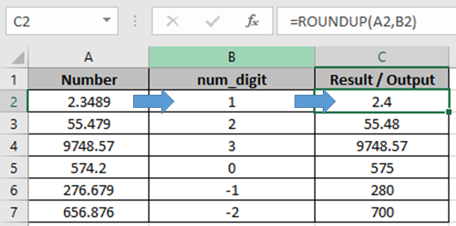
All of these might be confusing to understand. Let's understand how to use the function using an example. Here In one Column there are Numbers and in other, there are num_digits up to which the number to be rounded up.
Use the formula in C2 cell.
| =ROUNDUP(A2,B2) |
Explanation:
Here in C2 cell, the number will be round up to 1 decimal place.
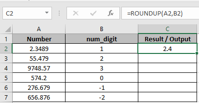
As you can see 2.4 is rounded up to 1 decimal place.
Copy the formula using Ctrl + D taking the first cell till the last cell needed formula.
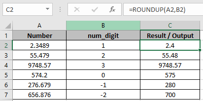
As you can see
| To get the number rounded up upto the nearest whole number, 0 is used default as num_digit |
ROUND to nearest hundred or thousand
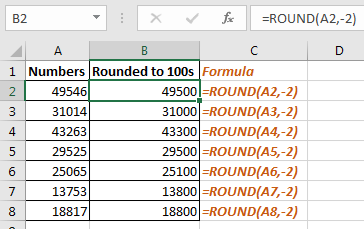
Here in range A2:A8, I have some numbers. I want to round them to 100. To do so I will write the formula below.
| =ROUND(A2,-2) |
Copy this in below cells.
How it works:
Actually when we pass a negative number to ROUND function, it round the numbers before decimal point.
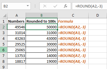
So to round to nearest 1000 we just need to replace -2 to -3 in formula.
Generic Formula to Round number to nearest 100
| =ROUND(number,-3) |
In same example, if we implement this formula we will get our numbers rounded to the nearest 1000.
This was quick tutorial of how how to round number to nearest 100 or 1000
Here are all the observational notes using the ROUND function in Excel
Notes :
Hope this article about How to use the ROUNDUP function in Excel is explanatory. Find more articles on rounding off values and related Excel formulas here. If you liked our blogs, share it with your friends on Facebook. And also you can follow us on Twitter and Facebook. We would love to hear from you, do let us know how we can improve, complement or innovate our work and make it better for you. Write to us at info@exceltip.com.
Related Articles :
How to use the FLOOR function in Excel | rounds down the number to the nearest specified multiple using the FLOOR function in Excel
Formula Round to nearest 100 and 1000 | Rounds off the given number to the nearest hundred or thousands using the ROUND function in Excel
How to use the ROUNDUP function in Excel | Rounds up the given number to the nearest num_digit decimal using the ROUNDUP function in Excel
How to use the ROUNDDOWN function in Excel | Rounds down the given number to the nearest num_digit decimal using the ROUNDDOWN function in Excel
How to use the MROUND function in Excel | rounds off the number to the nearest specified multiple using the MROUND function in Excel.
Popular Articles :
How to use the IF Function in Excel : The IF statement in Excel checks the condition and returns a specific value if the condition is TRUE or returns another specific value if FALSE.
How to use the VLOOKUP Function in Excel : This is one of the most used and popular functions of excel that is used to lookup value from different ranges and sheets.
How to use the SUMIF Function in Excel : This is another dashboard essential function. This helps you sum up values on specific conditions.
How to use the COUNTIF Function in Excel : Count values with conditions using this amazing function. You don't need to filter your data to count specific values. Countif function is essential to prepare your dashboard.
The applications/code on this site are distributed as is and without warranties or liability. In no event shall the owner of the copyrights, or the authors of the applications/code be liable for any loss of profit, any problems or any damage resulting from the use or evaluation of the applications/code.


