Multi Conditional Vlookup in Excel

Vlookup function in Excel is one of the most used functions. In this article, we will learn how to use Vlookup with multiple criteria.

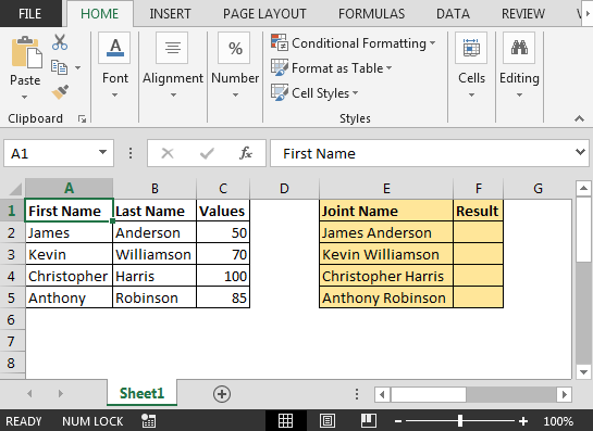
Question: I have a list of names in two columns & the third column contains values. I want Vlookup formula to incorporate the names with space in between & yield the values.

The function used in this tutorial will work on following versions of Microsoft Excel:

Excel 2013, Excel 2010, Excel 2007, Excel 2003

Following is the snapshot of Vlookup example:

• In cell F2 the formula is
• {=VLOOKUP(E2,CHOOSE({1,2},$A$2:$A$5&" "&$B$2:$B$5,$C$2:$C$5),2,0)}

Note: This is the array formula; use CTRL + SHIFT + ENTER keys together

• If the names combined with comma instead of space then the formula will be
• {=VLOOKUP(H2,CHOOSE({1,2},$B$2:$B$5&", "&$A$2:$A$5,$C$2:$C$5),2,0)}

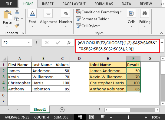
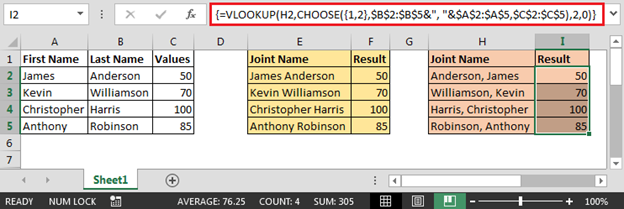
In this way, we can retrieve data meeting multiple conditions in Vlookup formula.

 

 

If you liked our blogs, share it with your friends on Facebook. And also you can follow us on Twitter and Facebook.
We would love to hear from you, do let us know how we can improve, complement or innovate our work and make it better for you. Write us at info@exceltip.com