

In this article, we will learn How to Use the INDEX and MATCH function to Lookup Value in Excel.
INDEX & MATCH function to replace vlookup function
We usually use the VLOOKUP function to find a value knowing the row Index and column number. For the VLOOKUP function we need to have the column number and row matching criteria and the most crucial thing the value to find out to be on the right of matching value. But the data doesn't always support that. Many times we need to just look up values not knowing the row or column index, just having the values to match. For example: finding the salary of an employee having Employee ID. In this we will look for Employee ID for row index and Salary for column index. Let's learn how we can do this lookup using INDEX & MATCH.
How to Solve the Problem?
For the formula to understand first we need to revise a little about the following functions
Now we will make a formula using the above functions. Match function will return the index of the lookup value1 in the row header field. And another MATCH function will return the index of the lookup value 2 from the column header field. The index numbers will now be fed into the INDEX function to get the values under the lookup value from the table data.
Generic Formula:
| = INDEX ( data , MATCH ( lookup_value1, row_headers, 0 , MATCH ( lookup_value2, column_headers, 0 ) ) ) |
data : array of values inside the table without headers
lookup_value1 : value to lookup in the row_header.
row_headers : Row Index array to lookup.
lookup_value1 : value to lookup in the column_header.
column_headers : column Index array to lookup.
Example:
The above statements can be complicated to understand. So let’s understand this by using the formula in an example
Here we have a list of scores gained by students with their Subject list. We need to find the Score for a specific Student (Gary) & Subject (Social Studies) as shown in the snapshot below.
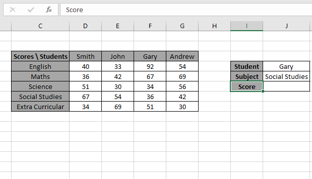
The Student value1 must match the Row_header array and Subject value2 must match the Column_header array.
Use the formula in the J6 cell:
| = INDEX ( table , MATCH ( J5, row, 0 , MATCH ( J4, column, 0 ) ) ) |
Explanation:
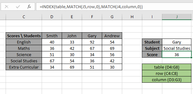
Here values to the formula is given as cell references and row_header, table and column_header given as named ranges.
As you can see in the above snapshot, we got the Score obtained by student Gary in Subject Social Studies as 36 . And it proves the formula works fine and for doubts see the below notes for understanding.
Now we will use the approximate match with row headers and column headers as numbers. Approx match only takes the number values as there is no way it applies on text values
Here we have a price of values as per the Height & Width of the product. We need to find the Price for a specific Height (34) & Width (21) as shown in the snapshot below.
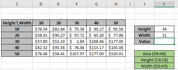
The Height value1 must match the Row_header array and Width value2 must match the Column_header array.
Use the formula in the K6 cell:
| = INDEX ( data , MATCH ( K4, Height, 1 , MATCH ( K5, Width, 1 ) ) ) |
Explanation:
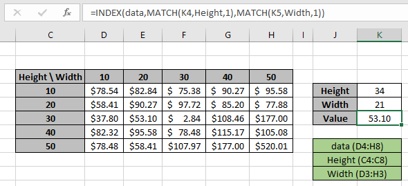
Here values to the formula is given as cell references and row_header, data and column_header given as named ranges as mentioned in the snapshot above.
You can also perform lookup exact matches using INDEX and MATCH function in Excel. Learn more about How to do Case Sensitive Lookup using INDEX & MATCH function in Excel. You can also look up for the partial matches using the wildcards in Excel.
As you can see in the above snapshot, we got the Price obtained by height (34) & Width (21) as 53.10 . And it proves the formula works fine and for doubts see the below notes for more understanding.
Notes:
Hope this article about How to use Use the INDEX and MATCH function to Lookup Value in Excel is explanatory. Find more articles on calculating values and related Excel formulas here. If you liked our blogs, share it with your friends on Facebook. And also you can follow us on Twitter and Facebook. We would love to hear from you, do let us know how we can improve, complement or innovate our work and make it better for you. Write to us at info@exceltip.com.
Related Articles :
Use INDEX and MATCH to Lookup Value : The INDEX-MATCH formula is used to lookup dynamically and precisely a value in a given table. This is an alternative to the VLOOKUP function and it overcomes the shortcomings of the VLOOKUP function.
Use VLOOKUP from Two or More Lookup Tables : To lookup from multiple tables we can take an IFERROR approach. To lookup from multiple tables, it takes the error as a switch for the next table. Another method can be an If approach.
How to do Case Sensitive Lookup in Excel : The excel's VLOOKUP function isn’t case sensitive and it will return the first matched value from the list. INDEX-MATCH is no exception but it can be modified to make it case sensitive. Let’s see how…
Lookup Frequently Appearing Text with Criteria in Excel : The lookup most frequently appears in text in a range we use the INDEX-MATCH with MODE function. Here's the method.
Popular Articles :
How to use the IF Function in Excel : The IF statement in Excel checks the condition and returns a specific value if the condition is TRUE or returns another specific value if FALSE.
How to use the VLOOKUP Function in Excel : This is one of the most used and popular functions of excel that is used to lookup value from different ranges and sheets.
How to use the SUMIF Function in Excel : This is another dashboard essential function. This helps you sum up values on specific conditions.
How to use the COUNTIF Function in Excel : Count values with conditions using this amazing function. You don't need to filter your data to count specific values. Countif function is essential to prepare your dashboard.
The applications/code on this site are distributed as is and without warranties or liability. In no event shall the owner of the copyrights, or the authors of the applications/code be liable for any loss of profit, any problems or any damage resulting from the use or evaluation of the applications/code.


