How to List Frequently Occurring Numbers in Excel

We know how to get the most frequently appearing number in excel. We use the MODE function. But if we want to list most frequently appearing numbers then this formula won't work. We will be needing a combination of excel functions to do this task.

Here is the generic formula to list the most frequently occurring numbers:

=MODE(IF(1-ISNUMBER(MATCH(numbers,expanding range,0)),numbers))

numbers: This is the range or array from which we need to get the most frequently appearing numbers.
expanding_range: It is an expanding range that starts from one cell above where you write this formula. For example, if right the excel formula in the cell B4 then expanding rang will be $B$3:B3.

Now, let us see this formula in action.

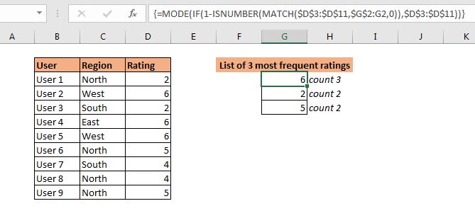
Example: Get 3 frequently appearing ratings.

So the scenario is this. We have some data on a survey in which users have rated our services. We need to get the 3 most frequently appearing ratings.

Write this formula in G3:

=MODE(IF(1-ISNUMBER(MATCH($D$3:$D$11,$G$2:G2,0)),$D$3:$D$11))

This is an array formula. Use CTRL+SHIFT+ENTER. Drag down this formula in three cells. And now you have your 3 most frequently occurring numbers.

Now that we have done it, let's see how it is working.

How does it work?

Here the idea is to exclude already extracted most frequently appearing numbers in the next run of MODE function. to do so we use some extra help from other excel logical functions.

To understand it let's have a look at the formula in cell G4. Which is:

=MODE(IF(1-ISNUMBER(MATCH($D$3:$D$11,$G$2:G3,0)),$D$3:$D$11))

The formula starts with the innermost function MATCH.

The MATCH function has lookup range D3:D11 (the numbers). The lookup value is also a range G2:G3 (expanded when copied down). Now, of course, G2 contains a text which is not in range D3:D11. Next, G3 contains 6. MATCH looks for 6 in range D3:D11 and returns an array of #N/A error and positions of 6 in range, which is {#N/A;2;#N/A;2;2;#N/A;#N/A;#N/A;#N/A}.

Now, this array is fed to the ISNUMBER function. ISNUMBER returns TRUE for numbers in the array. Hence we get another array as {FALSE;TRUE;FALSE;TRUE;TRUE;FALSE;FALSE;FALSE;FALSE}.

Next this array is subtracted from 1. As we know FALSE is treated as 0 and TRUE as 1. As we subtract this array from 1 we get an inverted array as {1;0;1;0;0;1;1;1;1}. This is the exact mirror image of the array returned by the ISNUMBER function.

Now, for each 1 (TRUE) MODE function runs. The MODE function gets an array {2;FALSE;2;FALSE;FALSE;5;4;4;5}. And finally, we get the most frequently appearing number in the array as 2. (Note that 5 and 4 both are occurring 2 times. But since 2 appeared first we get 2.

In G3, the ISNUMBER function returns an array of FALSE only. Hence the whole range is supplied to MODE function. Then mode function returns the most frequently appearing number in range as 6.

Another Formula

Another way is to use NOT function to invert the array return by ISNUMBER function.

{=MODE(IF(NOT(ISNUMBER(MATCH($D$3:$D$11,$G$2:G3,0))),$D$3:$D$11))}

So yeah guys, this how you can retrieve most frequently appearing numbers in excel. I hope I was explanatory enough. If you have any doubts regarding any function used in this formula, just click on them. It will take you to the explanation of that function. If you have any queries regarding this article or any other excel or VBA function, ask me in the comments section below.

Related Articles:

How to find frequently occurring numbers | Most frequently appearing numbers can be calculated using the MODE function of Excel.

Get most frequently appearing text in Excel | Learn how to get frequently appearing text in excel.

Lookup Frequently Appearing Text with Criteria in Excel | To get the most frequently appearing text in excel with criteria you just need to put an if condition before match function.

Retrieving the First Value in a List that is Greater / Smaller than a Specified Value | Learn how to lookup first value that is greater than a specified value. The generic formula to lookup is...

How to retrieve the entire row of a matched value| It is easy to look up and retrieve the entire row from a table. Let's see how can we do this lookup.

How to Retrieve Latest Price in Excel | To look up the latest price from a range you must have your data sorted. Once sorted use this formula...

Popular Articles:

50 Excel Shortcuts to Increase Your Productivity | Get faster at your task. These 50 shortcuts will make you work even faster on Excel.

The VLOOKUP Function in Excel | This is one of the most used and popular functions of excel that is used to lookup value from different ranges and sheets.

COUNTIF in Excel 2016 | Count values with conditions using this amazing function. You don't need filter your data to count specific value. Countif function is essential to prepare your dashboard.

How to Use SUMIF Function in Excel | This is another dashboard essential function. This helps you sum up values on specific conditions.