
To return the cell reference as text, we will use the Address Function in Microsoft Excel.
ADDRESS:- This function is used to creates a cell reference as text, given specified row and column numbers.
![]()
There are 4 options for abs_num:-
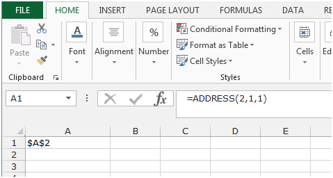
a) Absolute cell Reference (1) :- Address returns an absolute cell reference.
b) Absolute row/ Relative column (2) :- Address returns an absolute row with a relative column.
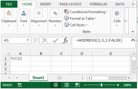
c) Relative row/ Absolute column (3) :- Address returns a relative row with an absolute column.
d) Relative (4) :- Address returns a relative cell reference.
For example:
We can use the ADDRESS function in 5 different ways.
| Syntax | Description |
|---|---|
| $C$2 | Absolute reference |
| C$2 | Absolute row; relative column |
| R2C[3] | Absolute row; relative column in R1C1 reference style |
| [Book1]Sheet1!R2C3 | Absolute reference to another workbook and worksheet |
| 'EXCEL SHEET'!R2C3 | Absolute reference to another worksheet |
Firstly, lets understand all the above ways of using the Address function.
Absolute Reference
The absolute reference is used where the column and row references are fixed.
Follow the below given steps:-
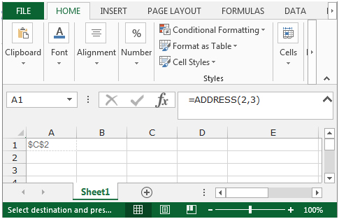
Absolute row; Relative column
The absolute row and relative column referencesare used, where only the row reference s fixed.
Follow the below given steps:-

Absolute row; relative column in R1C1 reference style
The absolute row and relative column references are used and the cell references are shown in the R1C1 format.
Follow the below given steps:-
Absolute reference to another workbook and worksheet
To show the absolute reference to another workbook and worksheet, follow the below given steps:-
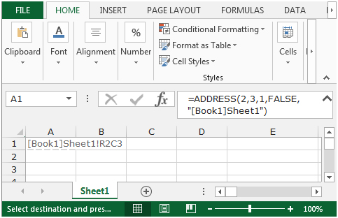
In this formula,the only difference is the last parameter where we get the cell references with the name of the workbook and worksheet. All other parameters are the same as explained above.
Absolute reference to another worksheet
To show the absolute reference to another worksheet, follow the below given steps:-
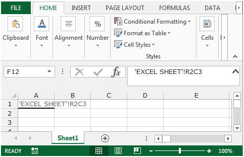
In this formula, we get the absolute cell reference with the name of the worksheet which is “EXCEL SHEET”.
These are the ways to get the Cell Reference as Text in Microsoft Excel.
![]()
If you liked our blogs, share it with your friends on Facebook. And also you can follow us on Twitter and Facebook.
We would love to hear from you, do let us know how we can improve, complement or innovate our work and make it better for you. Write us at info@exceltip.com
The applications/code on this site are distributed as is and without warranties or liability. In no event shall the owner of the copyrights, or the authors of the applications/code be liable for any loss of profit, any problems or any damage resulting from the use or evaluation of the applications/code.


I am trying to do this with a defined area in an array and INDIRECT does not work. Any ideas?
"This formula will return the contents of the cell:
=INDIRECT(ADDRESS(A1,A2,4,TRUE,A3))
INDIRECT changes a text address to one that can be used in a formula. But be aware this will only work if the workbook you're referencing is open."
This gave me the name of the cell I was after, but how do I get to the contents of that cell? Without directly referencing it, that is. I have a summary sheet and lots of data sheets, and want to just copy down a row when I add a data sheet.