
In excel conditional formula can be used to highlight the specific condition. In this article we will learn how to color rows based on text criteria, we use the option of “Conditional Formatting”.
This option is available in the “Home Tab” in the Styles group in Microsoft Excel 2010.
Conditional Formatting: -Conditional Formatting is used to highlight the important points with color in a report. We are formatting the data using colors, symbols, icons, etc based on certain conditions.
Let’s take an example to understand how you can conditional formatting row based on text criteria.
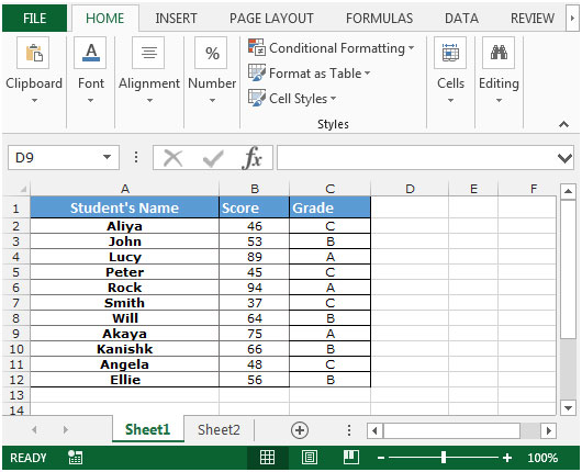
We have data in range A1:A10. Column C contains the grades. Now in column C we want to highlight the text with color. “A” grade should be highlighted with green color and “B” grade with blue color.
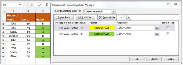
To color rows based on text criteria:


The output is shown below -
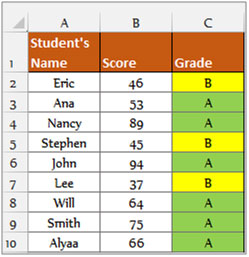
This is the way you can put conditional format based on color for specific text.
![]()
If you liked our blogs, share it with your friends on Facebook. And also you can follow us on Twitter and Facebook.
We would love to hear from you, do let us know how we can improve, complement or innovate our work and make it better for you. Write us at info@exceltip.com
The applications/code on this site are distributed as is and without warranties or liability. In no event shall the owner of the copyrights, or the authors of the applications/code be liable for any loss of profit, any problems or any damage resulting from the use or evaluation of the applications/code.


I think you've misspelled "SHIFT" in ?Select the range C2:C10 by pressing the key “CTRL+SHIT+Down arrow key”.
Oh! Sorry! SHIT happens.
I'm trying to set up a conditional formatting case as follows:
Look at the text in the cells of Sheet1 Column C
If any part of that text matches one of the words in Sheet2 Column B Rows 1-10,
then highlight the entire row in Sheet1 Column C where the match was found.
How the heck do I create a Conditional Formatting rule for that?
sdfgsdfg
"I am trying to create a golf scorecard. I would like to enter the number for each of the 18 holes. Then after playing the course I would enter my score for each hole. I would like to format the cell when I enter my score to change the backgroud color. If I am 1 over par it would change to asy red. If I was 1 under par it would change to green if 2 under par it would change to blue. Can you tell me how to do this in Excel.
Thanks for your help in advance."
"I need to know if it is possible to use Conditional formatting to compare a long list of competitor pricing in relation to our retail and then highlight the lowest retail of all of our competitors.
Any help would be appreicated.
Email jmcclain@pearison.com"
"The built in conditional formatting only allows for 3 sets of criteria.
If you want more you'll need to use VBA.
See here for an example:
http://rhdatasolutions.com/ConditionalFormatVBA/
This may have changed in newer versions of excel though (newer than excel 2000 anyway)."
I am trying to highlight data that is outside of the area 0 to 6. I also want it to highlight 0. How do I get it so it doesn't highlight blank cells???
Does the conditional formatting work for more than 3 Criteria?
"I am trying to create a golf scorecard. I would like to enter the number for each of the 18 holes. Then after playing the course I would enter my score for each hole. I would like to format the cell when I enter my score to change the backgroud color. If I am 1 over par it would change to asy red. If I was 1 under par it would change to green if 2 under par it would change to blue. Can you tell me how to do this in Excel.
Thanks for your help in advance."
"I need to know if it is possible to use Conditional formatting to compare a long list of competitor pricing in relation to our retail and then highlight the lowest retail of all of our competitors.
Any help would be appreicated.
Email jmcclain@pearison.com"
"The built in conditional formatting only allows for 3 sets of criteria.
If you want more you'll need to use VBA.
See here for an example:
http://rhdatasolutions.com/ConditionalFormatVBA/
This may have changed in newer versions of excel though (newer than excel 2000 anyway)."
"I am trying to highlight data that is outside of the area 0 to 6. I also want it to highlight 0. How do I get it so it doesn't highlight blank cells???
email me: john.morabito@ae.ge.com"
Does the conditional formatting work for more than 3 Criteria?