
In this article, we will learn how to determine in which quarter a specified date corresponds.
While working on reports, you have some dates & you want a formula which will return the date as Quarter number of the current year. Example: Jan 1, 2014 to be return as Quarter 1.
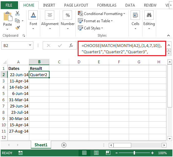
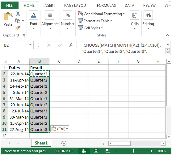
We will use a combination of CHOOSE, MONTH & MATCH functions together to make a formula that will return the date in a cell into Quarter number.
Choose: Returns the character specified by the code number from the character set for your computer. CHOOSE function will return a value from a list of values based on a given index number. Choose function uses index_num to return a value from a list.
Syntax = CHOOSE(index_num,value1,value2,...)
index_num: It specifies which value argument is selected. Index_num must be a number between 1 and 254 or a formula that contains number between 1 and 254. If index_num is less than 1, then Choose will return #VALUE!error.
value1 & value 2 are 1 to 254 value arguments from which CHOOSE will evaluate & return the result.
MONTH: This function returns the month (January to December as 1 to 12) of a date.
Syntax: =MONTH(serial_number)
serial_number: It refers to the date of the month that you are trying to find.
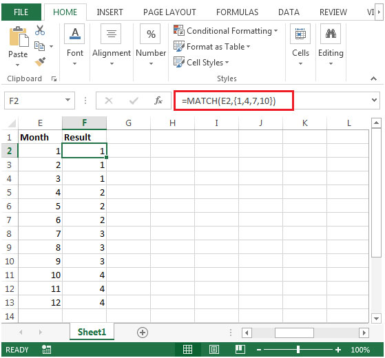
MATCH function searches for a specified item in a selected range of cells, and then returns the relative position of that item in the range.
Syntax =MATCH(lookup_value,lookup_array,match_type)
lookup_value: The value you want to look for
lookup_array: The table of data contains information from which you want to return the output.
match_type: 1,0 and -1 are three options.
1(Default): It will find the largest value in the range. List must be sorted in ascending order.
0: It will find an exact match
-1: It will find the smallest value in the range. List must be sorted in descending order.
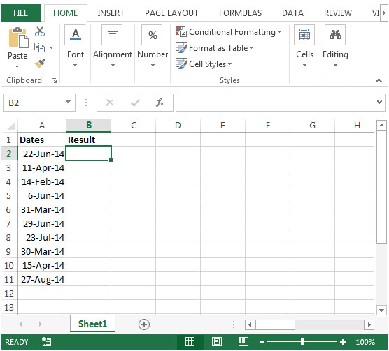
Let us take an example:
The applications/code on this site are distributed as is and without warranties or liability. In no event shall the owner of the copyrights, or the authors of the applications/code be liable for any loss of profit, any problems or any damage resulting from the use or evaluation of the applications/code.


Hi, thanks for this, it's very helpful! How would you tweet this when the quarters are misaligned. For example, I'm trying to align the date to the company's fiscal calendar, which Q1 is from May to Jul, Q2 is Aug to Oct. So in that case, the formula runs into error when the match formula becomes 2, 5, 8, ?. Thanks!