
For any reason, if you want to do some operation on a range with particular indexes, you will think of using INDEX function for getting array of values on specific indexes. Like this.

Let's Understand it With an Example.
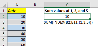
Here, I have a Rate column. I want to sum values at position 1,3, and 5. I write this formula in C2.
Surprisingly, INDEX function does not returns an array of values when we supply an array as indexes. We only get the first value. And SUM function returns the sum of one value only.
So how do we get INDEX function return that array. Well I found this solution on internet and I don’t really understand how it works, but it works.
The Generic Formula to get Array of Indexes
Range: It is the range in which you want to look for at given index numbers
Number: these are the index numbers.
Now let’s apply above formula to our example.
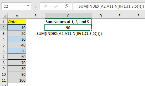
Write this formula in C2.
And this returns the correct answer as 90.
How It Works.
Well, as I said that I don’t know why it works and returns the array of numbers but here what happens.
IF(1,{1,3,5}): This part returns the array {1,3, 5} as expected
N(IF(1,{1,3,5})) this translates to N({1,3,5}) which again gives us {1,3,5}
NOTE: The N function returns the number equivalent of any value. If a value is not number convertable it returns 0 (like text). And for errors it returns error.
INDEX((A2:A11,N(IF(1,{1,3,5}))): this part translates to INDEX((A2:A11,{1,3,5}) and somehow this returns the array {10,30,50}. As you have seen earlier when write INDEX((A2:A11,{1,3,5}) directly in the formula it only returns 10. But when we use N and IF function it returns the whole array. If you understand it let me know in the comments section below.
How to use cell references for index values to get an array
In the above example, we hardcoded the indexes in function. But what if I want to have it from a range that may change. We replace {1,3,5} with range? Let’s try it.
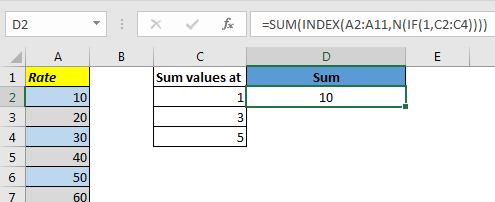
Here we have this formula in Cell D2:
This returns 10. The very first value of the given index. Even if we enter it as an array formula using CTRL+SHIFT+ENTER, it gives the same result.
To make it work add + or -- (double unary) operator before range and enter it as array formula.
This works. Don’t ask me how? It just works. If you can tell me how I will include your name and explanation here.
So we learned how to get an array from INDEX function. There’s some crazy stuff going on here in excel. If you can explain how it works here in the comments section below, I will include it in my explanation with your name.
Download file:
Related Articles:
Use INDEX and MATCH to Lookup Value
How to Use LOOKUP function in Excel
Lookup Value with Multiple Criteria
Popular Articles:
The applications/code on this site are distributed as is and without warranties or liability. In no event shall the owner of the copyrights, or the authors of the applications/code be liable for any loss of profit, any problems or any damage resulting from the use or evaluation of the applications/code.


This is great. Thanks! This has been added into the biggest beast of a function I have ever written and it seems to do the job perfectly.