
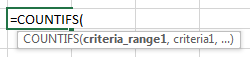
To count based on multiple criteria we use COUNTIFS function in Microsoft Excel.
Excel function COUNTIFS is used to count the entries in multiple ranges and with multiple criteria.
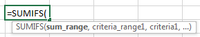
To sum based on multiple criteria we use te Sumifs function in Microsoft Excel.
SUMIFS:“SUMIFS” function is used to add the multiple criteria with multiple range.
Let’s take an example to understand how you can count based on multiple criteria.
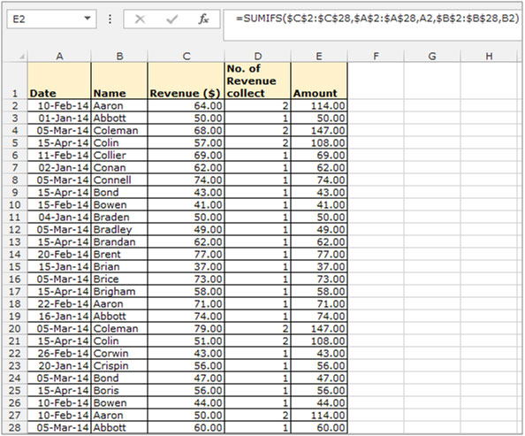
Example 1: We have data in the range A1: C28. Column A contains theDate, column B Name and column C contains Revenue.
In this example, we will count the number of collected revenue by a member on a particular date.

To Count the number for multiple criteria follow belowgiven steps:-

If you want to sum the Revenue based on these multiple criteria follow below mentioned steps:-
To convert the formula into value use the “Paste Special” option:-
![]()
If you liked our blogs, share it with your friends on Facebook. And also you can follow us on Twitter and Facebook.
We would love to hear from you, do let us know how we can improve, complement or innovate our work and make it better for you. Write us at info@exceltip.com
The applications/code on this site are distributed as is and without warranties or liability. In no event shall the owner of the copyrights, or the authors of the applications/code be liable for any loss of profit, any problems or any damage resulting from the use or evaluation of the applications/code.


I might sound very silly, but had been struggling to do this count of multiple criteria for at least 3 days and it has been running in the back of my mind all these 3 days. Thank you so much. It is way much simpler than what other websites I refereed to. Thanks.
"Hi Chris,
It won't work because the range that you are passing to the COUNTIF function is not a range:
MASTER!h(VALUE($R$2)):H(VALUE($R$3))
Rather than that expression, I am guessing that you want something like:
INDIRECT(""Master!h""&(VALUE($R$2))&"":H""&(VALUE($R$3)))
So your whole formula would read:
=COUNTIF(INDIRECT(""Master!h""&(VALUE($R$2))&"":H""&(VALUE($R$3))),$A3)
Even if that does not work exactly as you want, read up on the INDIRECT function and you should be able to work it out hopefully.
Does that help?
Alan."
"Can Anyone Tell Me Why The Following Statement Won't Work?
=COUNTIF(MASTER!h(VALUE($R$2)):H(VALUE($R$3)),$A3)"
"Hi Gunther,
I think this will do it.
Not very elegant, and I suspect that there is a better way, but I think it works (best to thoroughly test it though!)
Okay, if your data is in A1:A999 (say), then enter the following:
B1 = IF(ISERR(FIND(""photo"",A1)),0,FIND(""photo"",A1))
C1 = IF(ISERR(MID(A1,B1-1,1)="" ""),TRUE,MID(A1,B1-1,1)="" "")
D1 = IF(B1+5>LEN(A1),TRUE,MID(A1,B1+5,1)="" "")
E1 = AND(C1,D1)
Copy B1:E1 down to row 999 (or wherever your data ends).
You can now enter this formula wherever you like to get the count:
=COUNTIF(E1:E999,TRUE)
Probably best to test with a heavy dose of scepticism - I am not 100% sure that is what you want, but hopefully you can edit to suit if it is not.
Alan."
"Hi Alan,
e.g. content of cell A1 : this is a photo, A2: this is a photograph, A3: worldpressphoto, A4: the photo has been taken, A5: Photo
Result of the count should be 2 (photo in A1 and A4)
Regards,
Günther"
"Hi Gunther,
Could you give a (short) list of words as an example (including, say, ""photo"", and ""photograph"") alon with the search term, and the answer you would want so that we can get a clear idea.
Thanks,
Alan."
"Is there a way to count unique words in a range in Excel, e.g. unique word is photo but not ""photo"" in e.g. photograph should be counted.
The cells contain more than one word. "
"Hi Seth,
Sure - that is no problem.
Just put an IF statement around the outside of your array formula, and reference or calculate the alternative.
Remember that if any part of the formula is an array formula, you need to use Shift-Ctrl-Enter.
A simple way to do this is calculate both the array formula and non array formula in a calculation area, and then set up a simple IF statement to refer to the two cells in the calculation area depending on the answer to your decider.
Hope that helps,
Alan."
Is it possible to setup an array formula that is calculated only if a condition in another cell somewhere outside the array is met and if the condition is not met then another (non-array formula) is performed. Thanks.
"Hi Mark,
The FIND worksheet function is case sensitive.
For example:
If A1 and A2 contain ""Alan"" and ""Mark"" respectively, then:
{=SUM(1-(ISERROR(FIND(""a"",A1:A2))))} [=2]
{=SUM(1-(ISERROR(FIND(""A"",A1:A2))))} [=1]
Note that these are array formulae, and need to be entered with Ctrl-Shift-Enter.
Alan."
"Is there a way to use countif so it is case sensitive and distinguishes between a small ""s"" and a capital ""S"" ?
Great site by the way.
Cheers Mate."
Is there a way to count cells that are background formatted with a specific color? For example, I have a document that uses color codes to indicate what training sessions employees have taken. There are 6 different colors used. I would like to able to total the cells that have a certain color format.
Its typo mistake, fixed now.
I have tried this formula over and over and am not getting the result I am looking for. When I enter Cntl+Shift+Enter the bracket comes before the = so I'm wondering if that is the reason. Is there a way to enter the bracket in another area?
"the following sums next 7 columns on the right
ActiveCell.FormulaR1C1 = ""=SUM(RC[1]:RC[7])""
How do I sum next N columns on the right?
dim N=9
ActiveCell.FormulaR1C1 = ""=SUM(RC[1]:RC[&N&])"" 'will not work "
"It won't work because the range that you are passing to the COUNTIF function is not a range:
MASTER!h(VALUE($R$2)):H(VALUE($R$3))
Rather than that expression, I am guessing that you want something like:
INDIRECT(""Master!h""&(VALUE($R$2))&"":H""&(VALUE($R$3)))
So your whole formula would read:
=COUNTIF(INDIRECT(""Master!h""&(VALUE($R$2))&"":H""&(VALUE($R$3))),$A3)
Even if that does not work exactly as you want, read up on the INDIRECT function and you should be able to work it out hopefully.
Does that help? "
"Can Anyone Tell Me Why The Following Statement Won't Work? ,=COUNTIF(MASTER!h(VALUE($R$2)):H(VALUE($R$3)),$A3).
"
"I think this will do it.
Not very elegant, and I suspect that there is a better way, but I think it works (best to thoroughly test it though!)
Okay, if your data is in A1:A999 (say), then enter the following:
B1 = IF(ISERR(FIND(""photo"",A1)),0,FIND(""photo"",A1))
C1 = IF(ISERR(MID(A1,B1-1,1)="" ""),TRUE,MID(A1,B1-1,1)="" "")
D1 = IF(B1+5>LEN(A1),TRUE,MID(A1,B1+5,1)="" "")
E1 = AND(C1,D1)
Copy B1:E1 down to row 999 (or wherever your data ends).
You can now enter this formula wherever you like to get the count:
=COUNTIF(E1:E999,TRUE)
Probably best to test with a heavy dose of scepticism - I am not 100% sure that is what you want, but hopefully you can edit to suit if it is not. "
"e.g. content of cell A1 : this is a photo, A2: this is a photograph, A3: worldpressphoto, A4: the photo has been taken, A5: Photo
Result of the count should be 2 (photo in A1 and A4) "
Could you give a (short) list of words as an example (including, say, "photo", and "photograph") alon with the search term, and the answer you would want so that we can get a clear idea.
"Is there a way to count unique words in a range in Excel, e.g. unique word is photo but not ""photo"" in e.g. photograph should be counted.
The cells contain more than one word. "
"Sure - that is no problem.
Just put an IF statement around the outside of your array formula, and reference or calculate the alternative.
Remember that if any part of the formula is an array formula, you need to use Shift-Ctrl-Enter.
A simple way to do this is calculate both the array formula and non array formula in a calculation area, and then set up a simple IF statement to refer to the two cells in the calculation area depending on the answer to your decider.
Hope that helps, "
Is it possible to setup an array formula that is calculated only if a condition in another cell somewhere outside the array is met and if the condition is not met then another (non-array formula) is performed. Thanks.
"The FIND worksheet function is case sensitive.
For example:
If A1 and A2 contain ""Alan"" and ""Mark"" respectively, then:
{=SUM(1-(ISERROR(FIND(""a"",A1:A2))))} [=2]
{=SUM(1-(ISERROR(FIND(""A"",A1:A2))))} [=1]
Note that these are array formulae, and need to be entered with Ctrl-Shift-Enter. "
"Is there a way to use countif so it is case sensitive and distinguishes between a small ""s"" and a capital ""S"" ?
Great site by the way. "
Is there a way to count cells that are background formatted with a specific color? For example, I have a document that uses color codes to indicate what training sessions employees have taken. There are 6 different colors used. I would like to able to total the cells that have a certain color format.
Its typo mistake, fixed now.
I have tried this formula over and over and am not getting the result I am looking for. When I enter Cntl+Shift+Enter the bracket comes before the = so I'm wondering if that is the reason. Is there a way to enter the bracket in another area?