
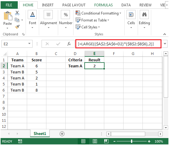
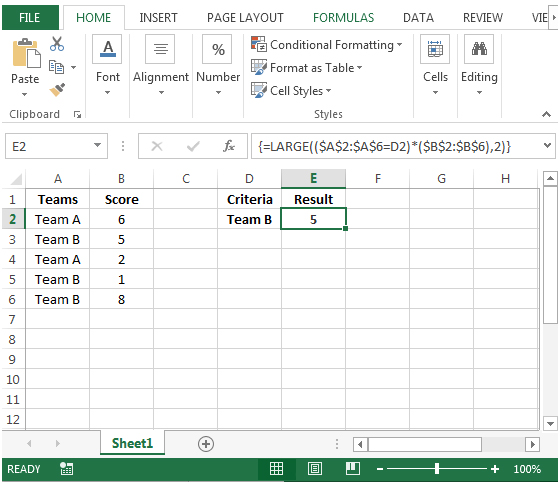
To find the nth highest score for a specified team, we can use the LARGE function to retrieve the result.
LARGE: Returns the k-th largest value in a data set. For example: the second largest number from a list of 10 items.
Syntax: =LARGE(array,k)
array: is an array or range of cells in a list of data for which you need to find the k-th largest value.
k: is the kth position from largest value to return in the array or range of cells.
Let us take an example:
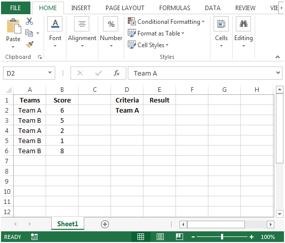
Column A contains couple of teams & column B contains their respective scores.We need a formula to derive the second highest score based on the selected team in cell D2.
The applications/code on this site are distributed as is and without warranties or liability. In no event shall the owner of the copyrights, or the authors of the applications/code be liable for any loss of profit, any problems or any damage resulting from the use or evaluation of the applications/code.


